The unit of observation is the field-year
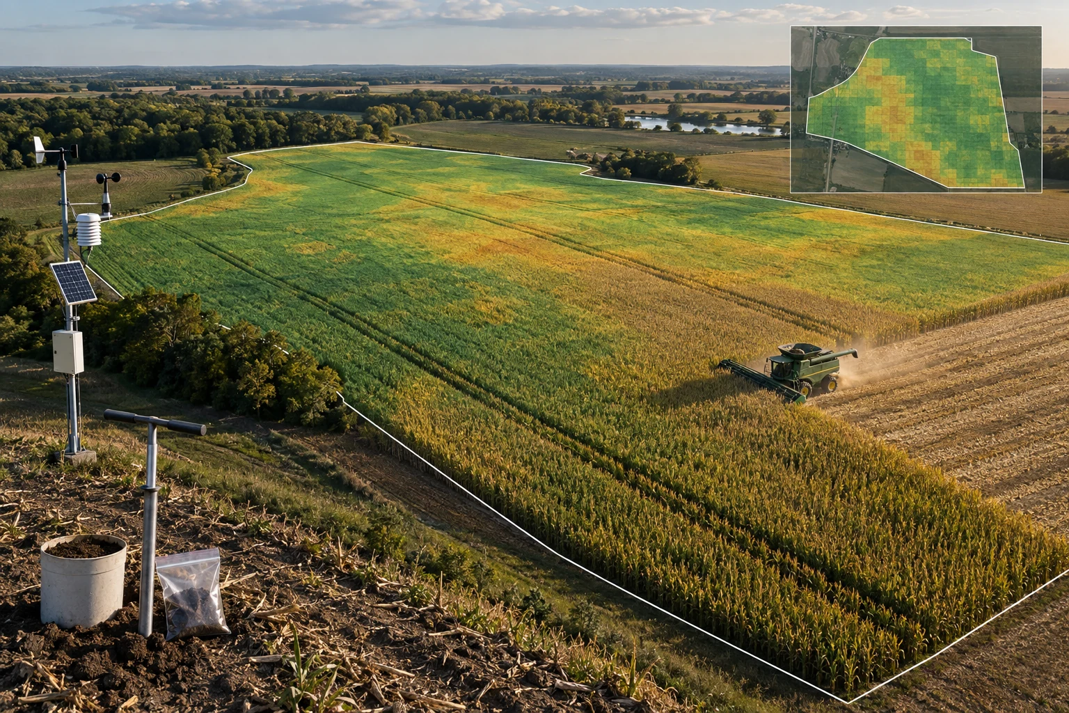
A yield model looks like a data-rich problem. Ten years of combine files, weekly satellite passes, soil grids, planting maps, applications, a rain gauge on the shop. Millions of rows. It is not a data-rich problem. Weather is the single largest driver of yield and every acre in a county shares the same weather in the same season, so a whole year of records tells you approximately one thing about how weather affects yield. Forty fields over four years is closer to a hundred and sixty observations than to two million, and the correlation between fields in the same year means the effective number is lower still.

Every consequence of importance follows from this. It is why a model with an impressive cross-validated score can be badly wrong the following August. It is why leaving out random rows is meaningless as a test and leaving out an entire season is the only honest one. It is why a model trained across three normal years will not know what to do in a drought, and why the year it most needs to be right is the year it has least seen.
It is also why the first honest question is not which algorithm, but how many field-years you have, spanning how many genuinely different seasons. If the answer is a dozen fields over three similar years, no modelling technique will rescue it, and an experienced agronomist will out-predict the software for another few seasons. That is not a reason to collect nothing. It is a reason to spend this year on measurement and boundaries and calibration rather than on a model that cannot yet exist.
You are probably here because
- You need a bushel estimate early enough to forward contract, and the current one is a guess
- A vendor showed a yield map that looked convincing and could not explain a single number on it
- You paid for variable-rate prescriptions and cannot tell whether they earned anything
- Two systems hold your field boundaries and they disagree about the acres
The last one sounds like housekeeping and is usually the item that has to be fixed before any of the others can be answered.
What imagery can see, and when it cannot
Satellite imagery is genuinely useful and routinely oversold. Three limits decide what a build can promise.
Clouds. A five-day revisit is not five-day data. Through the critical mid-summer growth window in a humid region it is common to end up with only a handful of usable scenes, and they will not be evenly spaced. Any product that assumes a clean weekly series has to be built to survive long gaps, and a model that quietly interpolates across a three-week hole is inventing the most informative part of the season.
Saturation. The standard greenness indices flatten once the canopy closes. In a good corn year that means the index stops separating an excellent field from a merely adequate one exactly when you want the distinction. Indices built to be less prone to this, and measures of when the canopy closed and how long it stayed green, carry more information than peak greenness on any single date.
Resolution against field geometry. Ten-metre pixels are fine for a hundred-acre field and poor near the edges. Thirty-metre pixels mixing crop with a treeline, a waterway or a road produce values that describe neither. Buffer every boundary inward before extracting anything, and expect to throw away a meaningful share of a small or irregular field.
| Source | Practical resolution and cadence | Good for | Where it disappoints |
|---|---|---|---|
| Public 10 m imagery Sentinel-2 class | Five-day revisit, far fewer clear scenes | Season-long curves, zone delineation, free at scale | Cloud gaps; edge pixels on small fields |
| Public 30 m archive Landsat class | Roughly two-week revisit, decades of history | Long baselines and multi-year trend work | Too coarse for within-field detail |
| Commercial daily imagery | Three to five metres, near-daily | Catching a short window; timing events | Subscription cost; radiometric consistency across scenes |
| Drone flights | Centimetres, whenever you fly | Stand counts, scouting, trial plots | Labour per acre; almost never a routine whole-farm layer |
| Radar imagery | Metres, sees through cloud | Filling gaps, structure and moisture signals | Harder to interpret; needs real processing work |
Your labels come off a combine, and they are dirty
The yield monitor is the label in every supervised model here, and raw monitor data is among the noisiest operational data in any industry we work in. The known failure modes are well documented in the agronomic literature and every one of them is present in a typical file.
Grain takes several seconds to travel from the header to the sensor, so yield is attributed to the wrong part of the field unless the delay is corrected. Start and end of pass produce partial header widths and a burst of implausible values. Turns and overlaps double-count. Moisture correction may or may not have been applied, and a file that mixes corrected and uncorrected passes is worse than either. Calibration drifts across a long harvest and often across operators, so two machines in the same field disagree by more than the effect you are trying to measure.
Cleaning this is a known procedure, not a research problem: remove the flow delay, drop the ramp at each end of a pass, remove overlapped passes using swath geometry, filter physically impossible speeds and yields, and normalise per machine and per day. It typically removes a substantial minority of the points and it changes field averages by amounts that matter. Do it once, keep the raw file forever, and record the version of the cleaning that produced any number anyone acts on.
Where the effort goes on a working yield model — our allocation
How a first build's hours actually divide, in our experience. The last row is the one every proposal is written about.
Rainfall is local and your nearest gauge is not close enough
Temperature interpolates reasonably across a county. Precipitation does not. A convective storm can drop two inches on one section and nothing four miles away, and if your weather source is an airport twenty miles off, that storm exists or does not exist in your data depending on luck. Since water is often the dominant yield driver, this single input can dominate model error.
What helps, roughly in order of cost. Use gridded radar-derived precipitation rather than a single station, and accept that it has its own biases. Put a real gauge on farms that matter and record its coordinates, because a gauge whose location is written as the farm name is not usable data. Where you have soil moisture probes, they are worth more than another year of imagery. And keep the irrigation records joined to the same field geometry, because on irrigated ground the applied water is a bigger input than the rain and it is often the record that lives only on a paper sheet in a pump house.
Three products get called yield prediction
An in-season bushel estimate for the whole operation. Used for marketing, storage and logistics. This is the most achievable and the most valuable. Field-average error in the range of eight to fifteen percent from mid-season is a fair expectation in a normal year, tightening as the season closes. Whether that is useful depends entirely on what you do with it, which is why the marketing or grain team should be in the room from the first meeting.
A within-field zone prediction. Used for variable-rate prescriptions. Much harder, because the model has to explain differences of a few bushels between parts of the same field while the label noise is of similar size. Stable multi-year yield patterns are real and worth mapping; a confident prediction for a specific zone in a specific season usually is not.
An attribution answer: did this practice pay. Not a prediction at all. It is an experiment, and treating it as a modelling problem is the most expensive mistake in this field.
Hold out a whole season, and report the bad year separately
Random row-wise cross-validation on a yield dataset produces numbers that are wrong by a wide margin, because rows from the same field-year are nearly duplicates and land on both sides of the split. Hold out entire years, one at a time, and report each year's error separately rather than averaging them. If one of those years was a drought or a wet spring, that year's number is the one that tells you whether the model is worth anything, and averaging it into three good seasons hides exactly the case you needed to see.
Send us one season of raw files and we will tell you what is in them.
Raw yield monitor exports, your boundary files, and the planting records for the same fields, to contact@precisionfederal.com. You get back what fraction of the points survive cleaning, how much the field averages move, where the boundaries disagree, and whether there is enough here to model at all. One business day, no charge.
contact@precisionfederal.comIf you want to know whether a practice worked, run a strip trial
The question we are asked most often is whether a product, a population, a hybrid or a rate earned its cost. Observational data cannot answer it, and no amount of modelling changes that. The acres that received the treatment were chosen, usually by an agronomist with good reasons, and those reasons are correlated with yield. The model then reports the agronomist's judgement back as the treatment effect.
The answer is old, cheap and boring: replicated strips, randomised, running the length of the field so they cross the soil variation, several pairs per field, repeated across fields and years. Modern equipment makes this nearly free to execute, and analysing it correctly means treating each strip pair as one observation rather than each pixel. A season of honest strip trials will tell you more than five years of retrospective analysis, and it is the only version of this work you can act on with confidence.
One statistical caution that costs people money: yield differences of one to three bushels are within the noise of a single field-year, whatever the map shows. Treat a small difference as a signal only when it repeats across replications and seasons.
What we would not build
- A yield model on fewer than about five genuinely different seasons presented as a decision tool
- Row-level cross-validation, which will report an accuracy you will never see again
- A prescription engine before the boundaries and monitor calibration are trustworthy
- A model whose weather input is one distant station in a region with convective rainfall
- Peak greenness as a single feature, when the canopy has been saturated since early July
- Treatment effects estimated from chosen acres and reported as though a trial had been run
- A dashboard with no interval, when the whole value of the estimate is in how sure it is
What a first build looks like
One off-season, in the order we would do it
Steps one and two are two-thirds of the work and all of the foundation. They are also the steps that get compressed when the schedule slips, which is how an operation ends up with a model built on acres it does not have and a harvest label nobody trusts. Step six has a hard deadline set by the planting calendar rather than by the project, and missing it costs a full year.
Before you commission anything
- You can state how many field-years you have and how many distinct seasons they span
- One authoritative boundary set exists, with a change history
- Yield files are cleaned by a documented procedure and the raw files are retained
- Evaluation holds out whole seasons and reports each year separately
- Imagery gaps are handled explicitly rather than interpolated away
- Precipitation comes from a gridded source or a gauge with real coordinates
- Every estimate carries an interval, and the interval is shown to whoever acts on it
- Practice questions are answered by replicated strips, not by retrospective comparison
- Someone has named the decision the estimate changes and when it must arrive
Bottom line
Yield prediction is a small-sample problem hiding inside a large file. The work that pays is unglamorous: one set of boundaries, one cleaning procedure, weather that reflects what fell on that field, imagery pipelines that survive a cloudy July, and evaluation that leaves out a whole season and tells the truth about the bad one. Field-average estimates for marketing and logistics are achievable now and worth real money. Within-field prescriptions are a longer road. Questions about whether a practice paid are experiments, and the strip trial is still the cheapest reliable answer anyone has found.
Frequently asked questions
For a field average in a normal season, error in the range of eight to fifteen percent from mid-season is a fair expectation, narrowing as harvest approaches. Extreme years are worse and are exactly the years you most want an answer. Within-field zone predictions are considerably less reliable, because the differences being predicted are similar in size to the noise in the yield monitor labels used to train on them.
Roughly five or more seasons that genuinely differ from one another, across as many fields as you can join reliably. The count that matters is field-years, not rows, and years that were all favourable count for less because they never show the model a stressed crop. With fewer, the useful work is measurement: fix boundaries, calibrate monitors, install gauges, and start replicated trials so next year's data is worth something.
For scouting, stand counts and trial plots, often yes, because resolution and timing are under your control. As a routine whole-farm data layer it rarely survives contact with the labour cost, and the flight schedule tends to collapse in the busy weeks that matter most. A common sensible split is public satellite imagery as the standing layer, with drone flights reserved for specific questions and trial ground.
Generally no, because the acres that received it were chosen for reasons connected to yield, and a model will report those reasons as the effect. Replicated randomised strips crossing the field's variation, repeated over fields and seasons, give an answer you can act on. Analyse the strip pair as the unit of observation rather than the pixel, and treat differences of a bushel or two in a single year as noise.
Yes. Most display software applies limited filtering and the raw record still contains flow-delay misattribution, end-of-pass ramps, overlapped passes and calibration drift between machines and days. Cleaning typically removes a substantial minority of points and moves field averages by amounts large enough to change a conclusion. Keep the raw files permanently and record which cleaning version produced any number that reaches a decision.