Sight distance from point clouds: turning LiDAR into a safety finding

A safety finding starts with a number an engineer can check

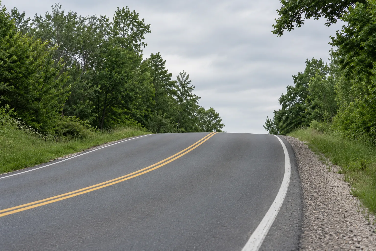
A driver cresting a hill into a curve lined with trees has a certain distance in which to see a stopped vehicle and stop. If that distance is shorter than the road requires at the speed people drive, the location has a sight distance deficiency, and an agency can act on it: clear vegetation, regrade a slope, add warning signs, or revisit the speed. Mobile LiDAR captures the shape of the road and everything beside it, which makes it possible to measure available sight distance along an entire corridor instead of at a handful of spots measured by hand. The point cloud does not produce a finding by itself. A defensible finding needs the right definition, the right inputs, a sound line-of-sight method and a record an engineer can check.

This guide walks through that path: the stopping sight distance definition, the inputs and where each comes from, how to compute available distance from a point cloud, how to compare it with the requirement, how to document the result, and the limits that come from the date the data was collected.

Stopping sight distance as the Green Book defines it

The AASHTO publication A Policy on Geometric Design of Highways and Streets, known as the Green Book, defines stopping sight distance as the distance a driver needs to perceive an object in the road, react, and brake to a stop before reaching it. It is the sum of two parts.

Brake reaction distance is the distance traveled from the moment the object becomes visible until the brakes are applied. The Green Book uses a brake reaction time of 2.5 seconds for design.

Braking distance is the distance traveled while decelerating to a stop. The Green Book uses a deceleration rate of 11.2 feet per second squared, a value most drivers can achieve on wet pavement while keeping control.

In U.S. customary units, with speed V in miles per hour, the level-road formula is: stopping sight distance = 1.47 × V × t + 1.075 × V² / a, where t is the brake reaction time in seconds and a is the deceleration rate. On a grade, the braking term becomes V² / (30 × ((a / 32.2) ± G)), where G is the grade as a decimal, positive for an upgrade and negative for a downgrade. Downgrades lengthen the stopping distance, and that matters on exactly the kind of crest-and-curve location this analysis tends to flag.

The definition also fixes the geometry of seeing. The driver's eye is taken as 3.5 feet above the road surface, and the object to be seen is 2.0 feet high. Those two heights are what turn a point cloud into a sight distance measurement: you are testing whether a line from a point 3.5 feet above the pavement to a point 2.0 feet above the pavement ahead is clear.

The inputs and where each one comes from

Every number in a sight distance finding should trace to a source. Writing this table down at the start of the project prevents the most common argument at the end of it.

Input	Value or form	Source
Driver eye height	3.5 ft above the pavement	Green Book
Object height	2.0 ft above the pavement	Green Book
Brake reaction time	2.5 s	Green Book
Deceleration rate	11.2 ft/s²	Green Book
Speed	Design speed, posted speed, or a measured operating speed	Agency design records, the posted limit, or a speed study; the choice must be stated
Grade	Percent, at each station	Profile computed from the classified ground points along the travel path
Travel path	Line along each lane with stations at a fixed interval	Lane lines extracted from the cloud, or the collection trajectory offset to the lane
Occluders	Terrain, vegetation, structures, barriers, signs	Classified point cloud, with moving and parked vehicles removed
Collection date and conditions	Date, season, leaf state	Collection metadata and imagery

Speed deserves a decision in writing. Comparing against design speed answers whether the road meets the standard it was designed to. Comparing against posted speed answers whether it supports the legal limit. Comparing against a measured operating speed, often the 85th percentile, answers whether it supports how people actually drive. Each is legitimate. A finding that does not say which one it used cannot be reviewed.

Preparing the point cloud

A sight line test is only as good as the points it tests against. Before computing anything, check the cloud's accuracy report and confirm the relative accuracy is good enough for the measurement. Vertical errors of even a few tenths of a foot matter when the question is whether a sight line clears a crest.

Then clean it. Remove points from vehicles that were moving or parked during collection, since they are not permanent occluders and will create false blockages. Remove noise points such as birds, dust and reflections. Classify what remains into ground, vegetation, structures, barriers and signs. Classification matters because the finding must name what blocks the view, and the remedy for a tree differs from the remedy for a hillside.

Computing available sight distance

The core method is a line-of-sight test repeated along the road.

Build the travel path. For each lane and direction, define a path that represents where drivers travel, usually the lane center. Place stations along it at a fixed interval, for example every 10 or 25 feet, chosen for the corridor. At each station, place the eye point 3.5 feet above the pavement surface.

Place target points ahead. From each station, place object points 2.0 feet above the pavement at increasing distances along the same path. On horizontal curves, the path follows the curve, so the sight lines cut across the inside of the curve, which is where roadside vegetation and cut slopes block the view.

Test each sight line. For each eye and target pair, check whether any point in the cloud lies within a small radius of the straight line between them. Ground points catch crest vertical curves. Vegetation and structure points catch roadside obstructions. The available sight distance at the station is the distance along the path to the farthest target that is still visible before the first blocked line.

Handle sparse obstructions carefully. A single point in thin brush may or may not represent a real obstruction. Use a rule, such as requiring a minimum number of points near the line, and apply the same rule throughout. State it in the method. A rule that is too strict will hide real problems behind gaps in the cloud. A rule that is too loose will flag every bare branch.

On horizontal curves, there is a useful cross-check. The Green Book gives the horizontal sightline offset needed for a given sight distance and curve radius: HSO = R × (1 − cos(28.65 × S / R)), with R and S in feet and the angle in degrees. Comparing the clear zone measured in the cloud with that offset is a quick sanity check on the line-of-sight results.

From point cloud to finding

The full workflow, in order, looks like this:

Comparing available with required

At each station, compute the required stopping sight distance from the chosen speed and the grade, then compare it with the available distance. Where available falls short, the station is deficient. Group consecutive deficient stations into segments, because an agency acts on a segment of road, not a station.

Report the size of the shortfall, not only whether one exists. A segment short by a few feet is a different priority from a segment short by a hundred. A second useful number is the speed the available distance actually supports, found by solving the formula for V. It translates the finding into the terms a traffic engineer and a council or commission understand.

Documenting a finding an engineer can defend

A finding will be reviewed by an engineer who did not run the analysis and may need to stand behind it in a public meeting or a claim. Give them everything needed to check it.

• Location: route, direction, lane, beginning and ending reference points or coordinates
• Required and available distance at each station, with the shortfall and the speed supported
• Every input and its source, including which speed was used and why
• The governing obstruction, classified and shown in a profile or plan view of the sight line
• Imagery from the collection showing the obstruction from the driver's position
• The collection date and season, with the leaf and crop state
• The method: station interval, line-of-sight radius, sparse-point rule and software version
• Field verification results for a sample of segments
• Limitations, stated plainly, such as data gaps or uncertain classification

Leave the remedy to the engineer. The analysis can say what blocks the view and by how much. Whether to clear vegetation, regrade, sign, or change the speed involves cost, right-of-way and policy judgments that belong to the agency.

Test the method before trusting the corridor

A line-of-sight engine is software, and software has bugs that look like findings. Before running a whole corridor, prove the engine on cases where the answer is already known.

A synthetic crest. Build a surface shaped like a parabolic crest vertical curve with a known algebraic grade difference A, in percent, and length L, in feet. With a 3.5 foot eye and a 2.0 foot object, the Green Book relationship for a crest where the sight distance S is shorter than the curve is L = A × S² / 2158, so the expected available distance is the square root of 2158 × L / A. Run the engine on the synthetic surface. If it does not return that distance within the station interval, something in the eye height, the target height or the occlusion test is wrong.

A synthetic curve. Place a wall of points at a known offset on the inside of a circular curve of known radius and compare the engine's answer with the horizontal sightline offset relationship. This exercises the path-following logic, which a crest test does not.

A measured site. Pick two or three real locations, measure available sight distance in the field with the standard targets and a measuring wheel or a survey instrument, and compare. Field measurement has its own error, so expect agreement within a stated tolerance rather than an exact match.

Keep these tests and rerun them whenever the code, the station interval or the occlusion rule changes. They are also the fastest way to answer a reviewer who asks how you know the software is right.

Seasonal and temporal limits

A point cloud is a snapshot. Vegetation is the biggest variable: a curve collected in winter with bare branches may show adequate sight distance that disappears in summer. Crops on adjacent farmland change height through the season. Snow banks narrow the clear area. Parked vehicles, temporary signs and construction materials come and go.

State the collection date and leaf state in every finding. Where vegetation governs, say so, and consider whether the result would change in another season. Where a decision depends on it, collect again in the critical season or verify in the field at that time of year. A finding that ignores season can be overturned by a single photo taken a few months later.

Beyond stopping sight distance

The same point cloud and line-of-sight engine support other sight distance checks, each with its own definition. Intersection sight distance looks across the approaches from a stopped or approaching vehicle. Decision sight distance applies where drivers face complex choices. Passing sight distance applies on two-lane roads. Each uses different eye and object assumptions and different required distances, taken from the Green Book and agency policy. Build the engine once, keep the definitions as configuration, and the work extends across all of them.

The habit that matters most is the same across all of them: define the requirement, trace every input, test against a clean cloud, and write the finding so another engineer can repeat it.

Frequently asked questions