
The work is mostly plumbing
Geospatial analytics answers questions where the answer depends on position. How much of this county burned. Which parcels sit inside the mapped floodplain. How many structures appeared between April and October. The modeling part is real, but projects rarely go sideways at the model. They go sideways because someone measured area in degrees, resampled a categorical raster with bilinear interpolation, or split train and test at random across pixels 10 meters apart. Our team treats the plumbing as the deliverable and the model as one component inside it.
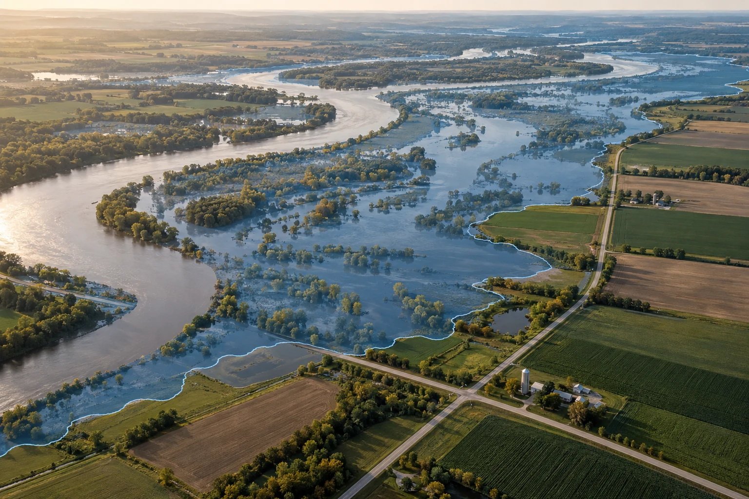
A tabular dataset assumes rows are independent; geospatial data violates that by construction. Spatial autocorrelation, the effect behind Tobler's 1970 formulation that near things are more related than distant things, is both the signal you want and the leak you have to defend against.
The second reason: a coordinate is not a number. It is a number plus a reference frame plus a datum plus a unit plus an axis convention, and most of that context lives somewhere other than the file you are reading. Federal work also governs those frames. OMB Circular A-16 assigns theme stewardship across agencies, and the Geospatial Data Act of 2018, enacted as Title VII of Public Law 115-254, put the Federal Geographic Data Committee and the National Spatial Data Infrastructure on statutory footing with reporting duties for covered agencies.
Where geospatial project risk concentrates
Editorial weighting from public sources and practitioner reading. Illustrative, not a measured statistic.
Three data models, three sets of rules
Raster. A grid of cells with a resolution, an origin, an affine transform, and a nodata sentinel. Continuous rasters (elevation, reflectance, temperature) tolerate interpolation. Categorical rasters (land cover, crop type, class masks) do not, and confusing the two is the most common silent corruption in a geospatial pipeline. Rasters are dense, so cost scales with area covered rather than with features of interest.
Vector. Points, lines, and polygons with attributes. Sparse, exact, and the right model when objects have identity: parcels, road segments, hydrants, boundaries. Vector work is dominated by topology. Are the rings closed. Do polygons self-intersect. Do adjacent parcels share edges or leave slivers. A layer that fails validity checks fails every geometric operation run on it afterward.
Point cloud. Irregular 3D returns from lidar or photogrammetry, in LAS or compressed LAZ, carrying classification codes, intensity, and return number. Usually an intermediate product: teams derive a bare-earth terrain model, a surface model, canopy height, or building footprints, then work in raster or vector from there.
Coordinate systems touch everything
Pick the analysis coordinate reference system first and write it down. EPSG:4326 is WGS 84 geographic, in degrees of latitude and longitude. It is a fine interchange format and a poor analysis frame, because a degree of longitude is about 111 kilometers at the equator and about 78 at 45 degrees north. Any length, area, or buffer computed in 4326 is wrong in a way that varies with where you are standing.
EPSG:3857, web Mercator, is the tiling frame for nearly every slippy map. It is conformal, so shapes are locally right, but the area scale factor grows roughly as one over the cosine of latitude, and acreage computed in it is badly overstated north of the mid-latitudes. For metric work, project into a local frame: a UTM zone (EPSG:326xx north, 327xx south for WGS 84, six degrees wide, scale factor 0.9996 on the central meridian) or the right State Plane zone. State Plane is usually what a survey or engineering customer already uses. The U.S. survey foot was deprecated at the end of 2022 in favor of the international foot, so older foot-unit definitions deserve a second look.
Axis order is the bug that keeps returning. The EPSG authority definition of 4326 is latitude then longitude. GeoJSON, per RFC 7946 published in 2016, mandates WGS 84 with longitude first. GDAL changed at version 3.0 and now honors authority axis order unless the code requests traditional GIS order. The symptom is unmistakable: your Iowa points land in Somalia. Every ingestion step should assert CRS and axis convention rather than inherit a driver guess.
Datums are the quieter version of the same problem. NAD 83 and WGS 84 differ by roughly one to two meters across the continental United States, invisible at 30-meter Landsat resolution and disqualifying at 10-centimeter lidar accuracy; NAD 27 to NAD 83 shifts run to tens of meters. Vertically, ellipsoid heights and NAVD 88 orthometric heights differ by the geoid separation, tens of meters in the CONUS. The National Geodetic Survey has been modernizing the National Spatial Reference System to replace both, so a long-lived product should record which frame its heights are in.
Federal data worth starting from
Most base layers a project needs already exist, funded, current, and free. USGS 3DEP publishes lidar and derived elevation nationally; the USGS Lidar Base Specification sets quality levels, with QL2 calling for 0.7-meter nominal pulse spacing and 10-centimeter RMSEz non-vegetated vertical accuracy. NAIP, run by the USDA Farm Service Agency, delivers four-band leaf-on aerial imagery at 60 centimeters, and 30 in places, on a repeating statewide cycle. Landsat 8 and 9 give 30-meter multispectral with an eight-day effective revisit between the pair, and USGS Collection 2 Level-2 surface reflectance is the analysis-ready form. Sentinel-2 adds 10-meter visible and near-infrared on a five-day revisit; one granule is 10,980 pixels square in the 10-meter bands.
On the vector side, Census TIGER/Line supplies boundaries, roads, and address ranges, the Census Geocoder resolves addresses at no cost, FEMA publishes the National Flood Hazard Layer, and HIFLD carries infrastructure layers at varying access tiers. For defense and intelligence work, the National Geospatial-Intelligence Agency is the functional manager for GEOINT and the source of authoritative foundation data.
The decisions that are expensive to reverse
Some choices cost an afternoon to change in week two and cost a full reprocessing run in month nine. We force these to the front of the schedule.
- The canonical analysis CRS. One frame for every stored geometry. Changing it later invalidates every cached tile, index, and precomputed distance.
- The spatial partition key. H3 resolution 9 averages about a tenth of a square kilometer: right for urban work, far too fine for a national rangeland product.
- Chunking and overview levels. Block size and pyramid depth are baked in at write time and govern every future read.
- The label taxonomy. Class definitions, minimum mapping unit, mixed-pixel handling. Relabeling costs more than remodeling, every time.
- Snapshot versus bitemporal. Adding valid time and transaction time to a snapshot store is a rewrite, not a migration.
- Nodata and masking convention. One sentinel value and one mask semantics, enforced at ingest.
Formats and the cloud-native stack
The last several years settled most of the format arguments. The Cloud Optimized GeoTIFF, now an OGC standard, is an ordinary GeoTIFF whose internal tiling and overviews let an HTTP range request pull one window without downloading the file. The SpatioTemporal Asset Catalog reached 1.0.0 in 2021 and makes those files findable by time, footprint, and property. GeoParquet released 1.0.0 in 2023, giving vector data columnar compression and predicate pushdown on object storage. Zarr covers arrays where time and band are first-class axes.
Shapefile still arrives constantly and still carries its original limits: a two-gigabyte ceiling per component file, attribute names truncated to ten characters, one geometry type per file, and no clean null representation. Accept it at the boundary and convert immediately. GeoPackage is the better single-file exchange when a customer needs something that opens in desktop GIS.
| Storage choice | Fits | Cost profile |
|---|---|---|
| COG on object storage | Imagery archives, elevation, derived continuous rasters | Cheap at rest; pay per range request, so chunk size drives the bill |
| GeoParquet on object storage | Large static vector: parcels, road networks, point observations | Very cheap; scan cost falls with good partitioning |
| PostGIS | Vector that changes, topology work, transactional joins | Always-on compute; index maintenance is the hidden line item |
| Vector tiles / PMTiles | Interactive map delivery at national scale | Fixed build cost, near-zero serve cost |
| Zarr | Time-series cubes, climate and weather stacks | Efficient for slicing across time; poor for one-off single-scene reads |
What "good" means numerically
Agree on the accuracy definition before writing code, and use the standards that already exist so the number is defensible outside the project. For positional accuracy, the FGDC National Standard for Spatial Data Accuracy and the ASPRS positional accuracy standards both express results as root mean square error at a stated confidence: horizontal accuracy at 95 percent equals RMSEr multiplied by 1.7308, vertical equals RMSEz multiplied by 1.9600. Those constants convert an internal error statistic into a claim a surveyor can check.
For thematic maps, report overall accuracy, per-class producer's and user's accuracy, and the confusion matrix. The 85 percent target traces to the Anderson land use and land cover classification system published by USGS in 1976 and remains the common bar; published National Land Cover Database assessments land in the 80s for detailed classes. Segmentation is scored with intersection over union, and building footprint extraction from high-resolution imagery is strong in the 0.80 to 0.90 range. Anything higher deserves a hard look at whether the test tiles were truly held out.
The rule teams skip most often: counting map pixels is a biased estimator of area. Olofsson and colleagues set out the good-practice method in Remote Sensing of Environment in 2014. Draw a probability sample of reference locations, build the error matrix, and produce area estimates with confidence intervals adjusted for classification error. A product reporting "142,000 acres changed" from raw pixel counts is unfalsifiable. The same product reporting 138,000 acres plus or minus 9,000 at 95 percent is something an agency can act on.
For monitoring systems, translate the score into the operator's unit: precision and recall at the chosen threshold, and false alarms per hundred square kilometers per revisit. An analyst who has to clear every alert cares about that second number.
Failure modes we check first
Every geospatial review our engineers run starts with the same short list, because these account for most of what goes wrong.
- Bilinear or cubic resampling applied to a categorical raster, inventing class values that do not exist in the legend
- Area or length computed in a geographic CRS, or acreage computed in web Mercator
- Nodata sentinels such as -9999 averaged into zonal statistics as if they were elevations
- Self-intersecting polygons from digitized sources failing GEOS operations, unrepaired by ST_MakeValid
- Random pixel-level train/test splits leaking across spatial autocorrelation
- Ellipsoid heights compared against NAVD 88 orthometric heights without geoid correction
- Scenes from different dates and sensors mosaicked without radiometric normalization, so the model learns the seam
- Segmentation inference run on non-overlapping tiles, producing visible edge artifacts at every tile boundary
The validation-split item separates a model that works from a model that reports that it works. Roberts and colleagues set out blocked cross-validation for spatially structured data in Ecography in 2017, and Ploton and colleagues showed in Nature Communications in 2020 that forest biomass models with excellent random-split performance collapsed under spatial cross-validation. If training and test samples share a neighborhood, the model can memorize the neighborhood. Spatial block or leave-one-region-out splits give a number that survives a new county.
On aggregation: the modifiable areal unit problem, named by Openshaw in 1984, means any statistic over aggregated zones depends on the zones chosen. Swap census tracts for hexagons and a correlation can change sign. When a deliverable aggregates to administrative units, our team tests two or more zonings and reports whether the finding holds.
Production: latency, cost, and monitoring
Serving at scale is a request-shape problem. A global web Mercator tile pyramid has four raised to the zoom level tiles; at zoom 14 that is 268,435,456, so pre-rendering all of them is a bad default. Render dense continuous data from COGs on demand and cache what people actually request; build vector tiles once and serve them as static objects.
Object storage economics reward chunk-size discipline. At AWS list prices, S3 GET requests run about $0.0004 per thousand and internet egress about $0.09 per gigabyte for the first ten terabytes a month in US regions. Small numbers, until a pipeline reads a 512-pixel window with forty range requests instead of two and request count rather than byte volume drives the bill. Matching read window to stored block size is the biggest cost fix our engineers make on inherited pipelines.
In the database, the classic PostGIS latency trap is a spatial predicate that cannot use the index. ST_DWithin is index-assisted; a filter written as ST_Distance below a threshold is not, and degrades to a full scan. With a GiST index and geometries in a projected CRS, point-in-polygon against a few million polygons should return in single-digit milliseconds. When it does not, the cause is usually a mixed-CRS join forcing on-the-fly transformation, or index bloat that VACUUM ANALYZE clears.
Monitoring means watching the geometry, not only the service. Instrument the ingest path for CRS of record, invalid and null geometry rates, nodata fraction per scene, and per-band reflectance distribution against the prior period. Imagery drifts with season, sun angle, and sensor changes, and a model that held its numbers all spring can lose several points of IoU when leaf-off imagery arrives. Cloud and shadow masks belong in the set, because rising cloud fraction explains far more sudden accuracy drops than model decay.
When a simpler method is the right answer
Many geospatial questions are geometry questions with exact answers, and a model adds cost, adds an approximation, and removes the ability to explain the result. Our default is deterministic geometry first, model second.
The question is "which features fall inside this boundary"
That is a spatial join, and PostGIS or DuckDB answers it exactly. Parcels intersecting a floodplain, hydrants within 300 meters of a structure, road segments crossing a jurisdiction: buffer and intersect give an answer an auditor can reproduce line by line.
The question is about vegetation, water, or burn severity
Normalized difference indices are hard to beat for cost and defensibility. NDVI from red and near-infrared, NDWI for surface water, and dNBR for burn severity underpin operational products including the Monitoring Trends in Burn Severity program. No labels, no training run, no GPU, and the thresholds are documented in the literature.
The question is flood extent from SAR
Open water has very low radar backscatter, making the histogram bimodal. Otsu thresholding on a calibrated SAR scene produces usable open-water extent in minutes. Reach for a segmentation network when the hard cases dominate: flooded vegetation, urban flooding under building shadow, wind-roughened water.
The question is a surface from scattered point samples
Inverse distance weighting or ordinary kriging usually beat a neural network on sparse observations, and kriging returns a variance surface the customer can map. In a decision product that is worth more than a marginally lower error with no uncertainty attached.
Models earn their place when the pattern is genuinely visual, the volume is beyond human review, or the signal sits in a combination of bands and textures no threshold captures. Structure extraction from imagery, crop type from a season-long spectral trajectory, damage assessment at disaster scale: those need learning. Counting parcels does not.
Markings, rights, and the derived layer
Federal geospatial work carries handling rules that shape the architecture. Imagery and derived products often arrive with limited-distribution markings or Controlled Unclassified Information categories, and CUI on a nonfederal system pulls in the NIST SP 800-171 control set, now at Revision 3, published in 2024. Commercial remote sensing is itself licensed: NOAA administers private remote sensing space systems under 15 CFR Part 960, whose 2020 rule restructured licensing into three tiers based on whether comparable capability already exists.
Rights in the derived layer are separate from rights in the source. FAR 52.227-14 governs rights in data generally, DFARS 252.227-7013 and 252.227-7014 cover noncommercial technical data and software on defense contracts, and SBIR-funded work carries its own protection under DFARS 252.227-7018. Settle in writing who holds which rights in the trained weights, the label set, and the output layers before first delivery. Labels are often the most valuable asset a project creates and the one teams forget to address.
Public-facing maps also carry a Section 508 obligation, and a map is not accessible simply because it renders. It needs keyboard operability, non-color-dependent encoding, and a textual equivalent for the underlying values.
How our team runs a geospatial build
The sequence is stable across projects. Fix the analysis CRS, units, and vertical datum in a config every job reads. Ingest to a normalized store with validity checks, nodata rules, and CRS assertions at the boundary. Set the accuracy definition and reference sample design before any modeling, so the target is a number rather than an adjective. Build the deterministic baseline first: it sets the bar the model has to clear and often turns out to be the deliverable. Then, where the problem earns it, train, evaluate with spatially blocked splits, and report area estimates with intervals.
That order is what makes the ambitious part possible. A modeling result is only worth what its coordinate frame, its validation split, and its accuracy definition are worth. Get those right and the rest of the work compounds.
Frequently asked questions
EPSG:4326 for interchange, EPSG:3857 only for tile delivery, and a local projected frame for anything measured. UTM works well for regional analysis; State Plane is usually right when the output feeds surveying or engineering. Record the choice in configuration and assert it at every ingest boundary.
Almost always a validation split that ignores spatial autocorrelation. Neighboring samples are near-duplicates, so a random split lets the model memorize the area. Spatially blocked or leave-one-region-out cross-validation gives a number that holds up in an unseen county.
For position, the FGDC National Standard for Spatial Data Accuracy or the ASPRS positional accuracy standards, reported as RMSE with the 95 percent multipliers of 1.7308 horizontal and 1.9600 vertical. For thematic maps, the full error matrix plus area estimates with confidence intervals from a probability sample.
Whenever the question has an exact geometric answer. Containment, proximity, overlap, and network distance are solved by spatial joins and buffers, and index thresholds handle much vegetation, water, and burn analysis. Models earn their place when the pattern is visual, the volume exceeds human review, or the signal spans bands and textures.