
Start with what is on the shelf
Every vendor pitch to a state DOT opens the same way: a model, a dashboard, a promise about prediction. The agency has heard it. What the agency actually wants to know is whether the vendor understands the five or six data holdings the department already maintains, what condition they are in, and which questions those holdings can answer without a new collection contract. That is a narrower conversation and a far more useful one. A department of transportation is a data organization that also builds roads. It has been collecting inventory, condition, volume, and crash records continuously for decades, under federal reporting rules that dictate the schema. Anyone proposing analytics into that environment should be able to name the files.
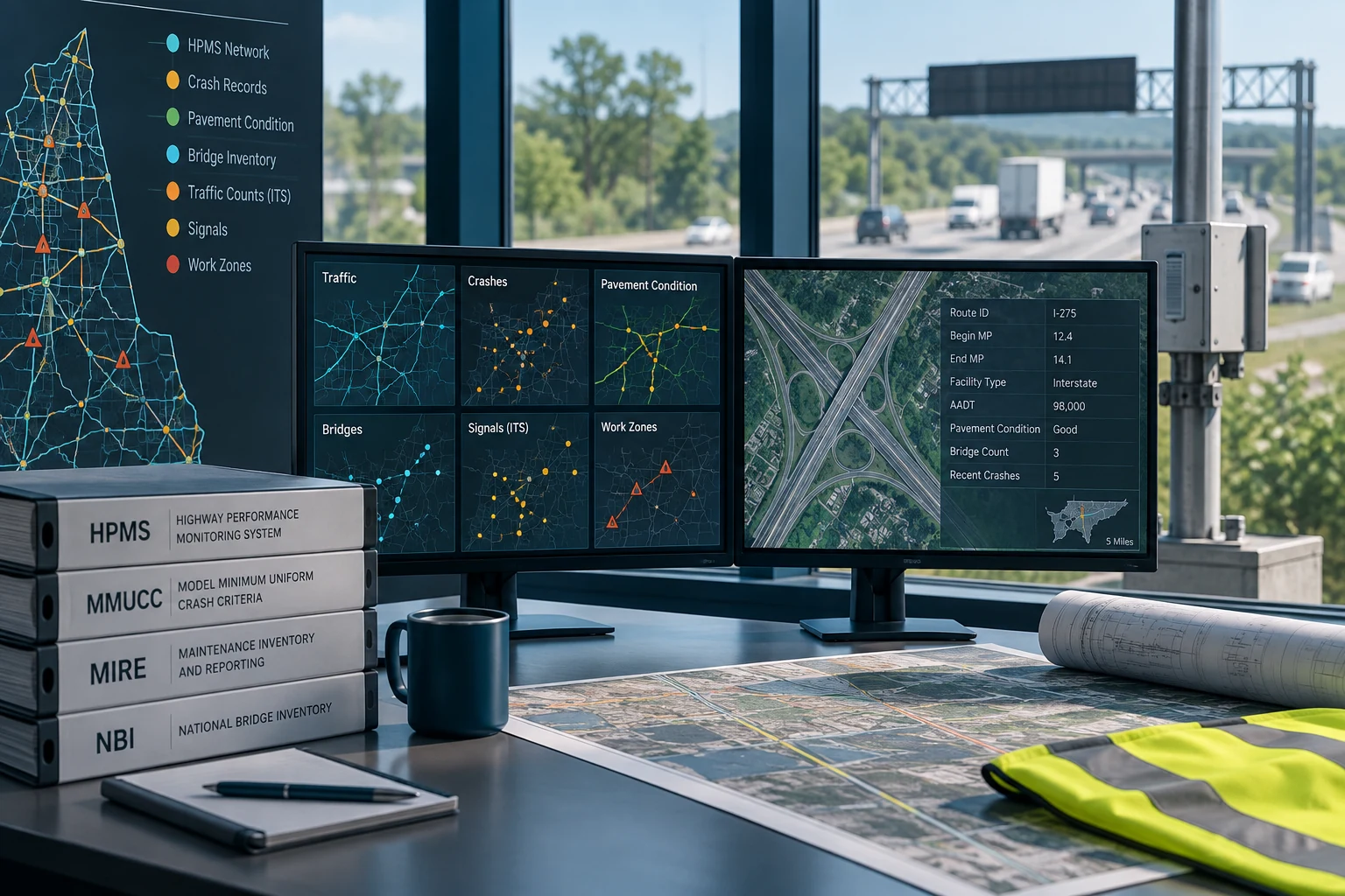
Our engineers work these holdings from the inside: the linear referencing system that ties them together, the reporting deadlines that shape them, and the quality problems that make a sound model produce a project list nobody can defend. What follows is the holdings in the order they usually matter, three uses that pay for themselves, and why the modelling choice rarely decides the result.
Modelling readiness by source, typical state DOT
Editorial weighting from public federal reporting requirements and open state data portals. Illustrative, not a measured statistic.
HPMS and the network underneath everything
The Highway Performance Monitoring System is the annual submittal every state makes to FHWA. It carries roadway extent, functional classification, through lanes, surface type, AADT, and condition items, some reported across the full network and some on a rotating sample panel. HPMS drives the Highway Statistics series, feeds apportionment formulas, and supplies the vehicle-miles-traveled denominator used in the federal safety performance measures. It is the closest thing to a canonical description of a state's road network.
What matters analytically is the restructure. HPMS 8.0 moved the submittal to a fully spatial, event-based model: attributes are events measured along routes in the state's linear referencing system rather than rows in a flat table. Under the All Road Network of Linear Referenced Data requirement, that LRS covers every public road in the state, not only the federal-aid network. If a department maintains a clean route-and-measure LRS, crash records, pavement runs, sign inventories, work zones, and traffic counts all segment onto the same geometry and join without a fuzzy spatial match. If the LRS is stale on locally owned roads, every downstream join inherits that error, and no amount of modelling repairs it.
Crash records, MMUCC, and what "location" means
The statewide crash file is built from police crash reports, moved through a records division, and closed for a calendar year some months after it ends. The Model Minimum Uniform Crash Criteria, now in its sixth edition, is voluntary guidance from NHTSA developed with FHWA and the Governors Highway Safety Association. It defines a minimum set of crash data elements and their permitted attribute values so that a rollover in one state means the same thing as a rollover in the next. States adopt it partially, which is the honest starting assumption for any multi-state analysis.
One piece of MMUCC is not voluntary. Under the federal safety performance measure rule at 23 CFR Part 490 Subpart B, states report five measures: fatalities, fatality rate per 100 million VMT, serious injuries, serious injury rate, and combined non-motorized fatalities and serious injuries. FHWA required states to use the MMUCC "Suspected Serious Injury (A)" definition for that reporting as of April 15, 2019. Any state that changed its injury scale around that transition has a discontinuity in its serious-injury time series, and a trend model fitted across the break will attribute a definitional change to a safety intervention.
Location is the field that decides whether crash data is usable. A crash coded to the wrong side of an intersection, to a parallel frontage road, or to a route that was renumbered lands in the wrong segment. It disappears from the corridor that would have been treated and inflates one that would not. Before any screening model runs, we measure the share of records carrying usable coordinates or route-and-measure values, the share geocoded from narrative text, and the offset distribution against the LRS. That diagnostic changes more project rankings than any choice of estimator.
MIRE, and the deadline sitting in front of every state
The Model Inventory of Roadway Elements is FHWA's listing of roadway and traffic attributes useful for safety analysis. Inside it sits a required subset: the MIRE Fundamental Data Elements, 37 items covering roadway segments, intersections, and interchange ramps, with a reduced set applying to locally owned paved roads and to unpaved roads. Segment items include surface type, lane and shoulder width, median type, AADT and its year. Intersection items include the type of traffic control and the number of approach legs.
September 30, 2026: MIRE fundamental data elements on all public roads
The Highway Safety Improvement Program rule at 23 CFR 924.11(b) requires each state to have access to a complete collection of the MIRE fundamental data elements on all public roads by September 30, 2026. For most departments the gap is not the state-maintained system. It is the county and municipal mileage, where the inventory was never assembled to a common schema. HSIP funds under 23 U.S.C. 148 and State Traffic Safety Information System grants under 23 U.S.C. 405(c) are both available for the collection work.
That deadline is the largest single driver of roadway-inventory work in the states right now, and it is where machine learning earns its place quickly. Extracting lane counts, shoulder widths, median type, intersection control, and lighting presence from mobile LiDAR and 360-degree imagery is a mature computer-vision problem, and the alternative is a field crew driving several thousand miles of county road. The deliverable is the extraction plus a per-attribute accuracy report against a manually coded validation sample, so the department can tell FHWA how good the inventory is.
Pavement and bridge condition
Pavement condition arrives from a data collection vehicle running an inertial profiler and imaging system. The International Roughness Index is computed from the measured longitudinal profile; cracking percent, rutting on asphalt, and faulting on jointed concrete complete the federal set under 23 CFR Part 490 Subpart C. The thresholds have teeth: if more than five percent of a state's Interstate lane-miles fall in the Poor category, the state must direct National Highway Performance Program funds to Interstate pavement. Part 490 also requires a pavement data quality management program, so the department already owns a written definition of acceptable error and a repeat-run verification process. That is the ready-made basis for judging whether a deterioration model's inputs are stable.
Bridges are the better-documented asset. The National Bridge Inventory holds more than 620,000 structures nationally, inspected under the National Bridge Inspection Standards at 23 CFR Part 650 Subpart C. The 2022 NBIS final rule introduced risk-based inspection intervals as an alternative to a fixed routine cycle, and FHWA's Specifications for the National Bridge Inventory replaced the 1995 Recording and Coding Guide, changing item names and coding. On the National Highway System, element-level condition quantities under the AASHTO Manual for Bridge Element Inspection give quantity by condition state for each element rather than a single deck, superstructure, and substructure rating. Bridge condition has its own federal floor: exceeding ten percent of NHS bridge deck area in Poor condition for three consecutive years forces NHPP funds toward bridges under 23 CFR 490.411.
| Holding | Refresh | The failure mode that bites |
|---|---|---|
| HPMS + LRS | Annual submittal | Route renumbering and stale local-road geometry break every join built on route-and-measure. |
| Crash file | Continuous, year closes months later | Location coding error moves crashes off the segment that would have been treated. |
| Pavement condition | Annual or biennial by network | Distress definitions and collection vendors change; the trend breaks at the contract boundary. |
| Bridge inspection | Routine cycle, risk-based intervals | Ordinal ratings carry real inspector-to-inspector variability, so small changes are noise. |
| ITS and signal feeds | Sub-second to 5 minutes | Detector and sensor failures are silent; bad data looks like a traffic pattern. |
| Work-zone activity | Event driven | Planned dates rarely match actual lane closures, so before-and-after windows are wrong. |
ITS feeds: counts, signals, and roadside sensors
Traffic monitoring follows FHWA's Traffic Monitoring Guide. A modest number of continuous count stations run all year, recording hourly volume, vehicle classification under the 13-category federal scheme, and at weigh-in-motion sites, axle weights. Those stations produce the seasonal and axle-correction factors that convert thousands of short-duration counts into AADT. States submit the continuous data to FHWA through the Travel Monitoring Analysis System. This is the strongest, longest, cleanest time series a DOT owns, and it is underused: it supports demand forecasting, seasonal freight patterns, and the exposure denominator for every safety model in the building.
Signal systems are the second feed. A modern controller writes a high-resolution event log at tenth-of-a-second resolution, one row per event code with its parameter and timestamp, which is what Automated Traffic Signal Performance Measures are computed from: arrivals on green, split failures, queue behavior, pedestrian delay, and detector health. Field and center communications ride NTCIP, with 1202 for actuated signal controllers, 1203 for dynamic message signs, and 1204 for environmental sensor stations. Probe-based travel times on the National Highway System arrive as the National Performance Management Research Data Set in five-minute bins, which is what the Part 490 reliability measures are built on.
The unglamorous truth about ITS feeds is that detector and sensor health is the first deliverable. A loop failed stuck-on reports a plausible volume. A radar unit knocked out of alignment reports a plausible speed. Both feed a performance dashboard and quietly corrupt it. An anomaly monitor that flags each device against its own history and against its neighbors is cheap to build and pays back faster than anything downstream.
Work zones and the exchange feed
Work-zone data used to live in a spreadsheet in a district office. The Work Zone Data Exchange specification changed that by defining a common GeoJSON feed for active work-zone events, with location, lane impacts, and start and end times, published so that navigation providers, connected vehicles, and the department's own 511 service read the same record. The regulatory backdrop is the Work Zone Safety and Mobility Rule at 23 CFR Part 630 Subpart J, which requires a state policy, significant-project determinations, and the use of field observations and work-zone crash data to manage impacts.
Pair a work-zone feed with probe travel times and the department can finally measure what a closure cost: queue length and duration by hour, diversion onto parallel routes, and delay in vehicle-hours priced with the department's own user-cost values. That supports lane-rental provisions, night-work decisions, and the impact analyses the rule already asks for. The catch is in the table above. Planned closure windows and actual closure windows differ, so any before-and-after computed on planned dates will misreport, and reconciling the feed against probe or detector evidence of the real closure is part of the job.
Three uses that pay for themselves
Network screening for safety. The AASHTO Highway Safety Manual predictive method is the accepted approach: a safety performance function estimates crashes for a site given its traffic volume and geometry, crash modification factors adjust for features, and an empirical Bayes step combines the prediction with observed history to correct for regression to the mean. Sites are then ranked by potential for safety improvement, the gap between expected and predicted crashes. On low-volume and locally owned roads where crashes are too sparse to rank sites, systemic screening substitutes: find the risk features associated with severe crashes statewide, then flag every location carrying them whether or not a crash has happened there yet. Both survive scrutiny because the reasoning is inspectable site by site.
Deterioration forecasting for the asset management plan. Every state maintains a Transportation Asset Management Plan for NHS pavements and bridges under 23 U.S.C. 119(e) and 23 CFR Part 515, and the plan must contain life-cycle planning, risk management, a financial plan, and investment strategies. Deterioration models are required content, not an enhancement. The work is forecasting condition forward under alternative funding levels with honest uncertainty bands, then reporting how much of the network sits within reach of the federal floors. Markov transition models remain the workhorse for bridges and are easy to defend; survival models handle treatment timing well. Gradient-boosted models often fit slightly better and lose the room if the ranking cannot be explained.
Work-zone and corridor impact measurement. Described above, and the shortest path from a pilot to a number a district engineer trusts, because the department can check the result against what its own staff watched happen.
Why data quality decides it, not model choice
The modelling literature for these problems is settled enough that the choice among reasonable estimators moves the answer far less than five recurring data problems.
The exposure denominator carries error. AADT on most segments is a 48-hour count factored by seasonal and axle adjustments borrowed from the nearest continuous counter that shares a traffic pattern. On an instrumented urban arterial that estimate is tight. On a rural county road whose seasonal profile matches no nearby station, it is not, and it sits in the denominator of every crash rate and in the input to every safety performance function.
Ordinal condition ratings are noisier than they look. FHWA's study of visual bridge inspection reliability (FHWA-RD-01-020, 2001) found that individual condition ratings varied substantially across inspectors examining the same structure, with roughly two-thirds falling within one point of the average and about ninety-five percent within two. A model that treats a one-point change as a real deterioration event is largely fitting inspector variation.
The reference frames move. HPMS 8.0 restructured the submittal. SNBI renamed and recoded bridge items. MMUCC editions change attribute values, and states adopt them at different times. Crash reporting thresholds for property-damage-only collisions differ by state and have been raised over the years, which changes the count without changing the road. A time series assembled across any of those boundaries needs an explicit break, and most raw extracts do not carry one.
Severe outcomes are rare. Fatal crashes are a small fraction of reported crashes. A classifier optimized for overall accuracy predicts "not severe" everywhere and scores beautifully. Calibrated probabilities, count models with the right variance structure, and evaluation at the operating point the agency will actually use are what make the output usable.
The result has to be defensible in public. Project selection under HSIP is reviewed by FHWA, published in an annual state safety report, and questioned by legislators, county engineers, and residents who want to know why their intersection ranked eleventh. A model whose ranking can be traced to volume, geometry, crash history, and a named crash modification factor wins that room. A model that returns a score and no reasoning loses it, whatever the cross-validation says. We build for the second audience from the first sprint, and the design constraint improves the analysis rather than limiting it.
How our team runs the first ninety days
Engagement pattern, transportation data work
Step three is the one clients remember. Reproducing a published figure, a pavement condition percentage or a fatality rate, forces every definitional question into the open in week five instead of month nine. When the two numbers differ, one of us has found something worth knowing.
How this work gets bought
State DOTs buy analytics several ways, and the path changes the schedule more than the scope does. On-call and task-order contracts for planning, traffic engineering, and IT services are the fastest route for a defined study. Engineering and design related services on federal-aid projects follow qualifications-based selection under the Brooks Act and 23 CFR Part 172, so price is negotiated after selection and consultant prequalification is often a precondition. Software and data services often move through central state IT procurement or a cooperative vehicle instead. Local agencies spending federal funds work under 2 CFR Part 200. Safe Streets and Roads for All grants fund safety action plans and the data work behind them, while HSIP and 405(c) funds sit behind most state-level data improvement.
Precision Federal builds AI, data, and software systems for federal, state, and local customers, and works as a prime or as a subcontractor to the engineering firms that hold the on-call contracts. Our team includes licensed professional engineers alongside the data and machine-learning engineers, which matters when a deliverable has to line up with an agency's own standards and get signed.
Bottom line
The data a state DOT holds is better than most outside firms assume and messier than inside staff will claim in a first meeting. It is well-specified, federally structured, and long enough to model. It also carries location error, definitional breaks, silent sensor failures, and rating noise that decide the answer before any estimator is chosen. Teams that spend their first month on the joins, the device health, and the series breaks produce project lists that hold up in a public meeting. Teams that spend it on model selection produce a demo.
Frequently asked questions
A linear referencing system covering all public roads, the annual HPMS submittal, a statewide crash file, pavement condition from profiler runs, bridge inspection records under the National Bridge Inspection Standards, traffic counts from continuous and short-duration stations, signal controller event logs, and increasingly a work-zone data feed. Most departments can produce all of it without a new collection contract.
They are the 37 roadway, intersection, and ramp attributes from FHWA's Model Inventory of Roadway Elements that states must collect for safety analysis, with a reduced set for locally owned paved and unpaved roads. Under 23 CFR 924.11(b), states must have access to a complete collection on all public roads by September 30, 2026.
MMUCC itself is voluntary guidance from NHTSA, FHWA, and GHSA that standardizes crash data elements and attribute values across states. One piece is mandatory: for federal safety performance reporting under 23 CFR Part 490, states have been required to use the MMUCC "Suspected Serious Injury (A)" definition since April 15, 2019.
Usually location coding and regression to the mean. Crashes assigned to the wrong segment shift the ranking, and sites that had a randomly high year look worse than they are. The empirical Bayes step in the Highway Safety Manual method exists to correct the second problem; a location-coding audit against the LRS is the fix for the first.
Yes for many attributes. Lane and shoulder configuration, median type, intersection control, lighting, and roadside features extract reliably from mobile LiDAR and 360-degree imagery. The deliverable should include per-attribute accuracy measured against a manually coded validation sample, plus a review queue for low-confidence extractions, so the agency can report how good the inventory is.