
Start with what already exists
There are roughly 50,000 community water systems in the United States, and more than nine in ten serve fewer than 10,000 people. At the large end a utility runs its own control room, certified laboratory, and GIS department. At the small end it is two certified operators, a SCADA screen, and a spreadsheet. Both ends face the same four questions: which pipe do we replace first, where is the water going, is this month's compliance number defensible, and can we prove all three to the state. The data to answer them almost always exists already. Nobody needs a new sensor network first.
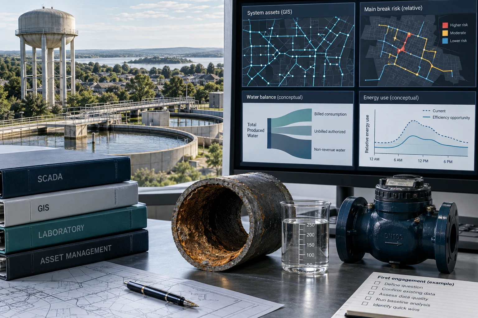
The pressure behind those questions is capital. EPA's 7th Drinking Water Infrastructure Needs Survey and Assessment, published in 2023, put the twenty-year national need at $625 billion. The Bipartisan Infrastructure Law routed roughly $50 billion through EPA's State Revolving Funds, including about $15 billion for lead service line replacement. A utility whose rehabilitation budget covers half a percent of its mains a year is making a ranking decision annually, and the quality of that ranking is worth more than any model architecture argument.
Our engineers work a municipal system the same way we work a federal one: inventory the sources, measure what is in them, pick the one decision worth real money, and build the thinnest pipeline that carries it into production. Everything below is what that inventory usually finds.
The four systems that hold the answers
SCADA and the historian. Plant and network telemetry lands in a PLC or RTU layer and is archived in a historian: AVEVA PI, GE Proficy, Ignition, Rockwell FactoryTalk, or an open time-series store. Field communication runs on Modbus TCP, DNP3 (IEEE 1815), or OPC UA (IEC 62541), with MQTT and Sparkplug B common on newer cellular telemetry. A mid-size utility carries 5,000 to 50,000 tags: tank levels, pump status and runtime, discharge pressure, flow, turbidity, chlorine residual, blower speeds, influent flow.
Metering and billing. Most utilities over 20,000 connections now have hourly or 15-minute interval reads for at least part of the service area. Reads land in a head-end system and flow into a customer information system such as Tyler Munis or Harris NorthStar. The meter-to-account-to-address mapping in that chain is where the reconciliation pain lives.
GIS and maintenance records. Pipe geometry, material, diameter, and install year live in Esri, often in the Utility Network data model. Work history lives in a CMMS: Cityworks, Cartegraph, Maximo, or a homegrown ticket table. Break records are the most valuable asset dataset a utility owns and almost always the messiest.
Laboratory and compliance. Sample results live in a LIMS or, more often than vendors admit, in Excel workbooks by year. They feed monthly operating reports to the state, Discharge Monitoring Reports through NetDMR under the NPDES electronic reporting rule at 40 CFR Part 127, and the annual Consumer Confidence Report required by 40 CFR Part 141 Subpart O.
| Source | Typical shape at a 100,000-connection utility | Useful latency |
|---|---|---|
| SCADA historian | 20,000 tags, 1 to 10 second local scan, 1 to 15 minute remote telemetry; deadband compression stores 2 to 10 percent of raw samples | 1 to 5 minutes for advisory use |
| AMI interval reads | 100,000 meters at 15-minute intervals = 9.6 million rows a day, about 3.5 billion a year, 60 to 120 GB a year in compressed Parquet | Daily batch; hourly for continuous-flow alarms |
| GIS asset inventory | 800 to 1,500 miles of main split into 15,000 to 40,000 segments; install year missing or estimated on 20 to 50 percent | Quarterly refresh |
| CMMS work orders | 30,000 to 200,000 historical records, failure cause in free text, 10 to 20 years of usable break history | Nightly |
| LIMS and compliance | Thousands of results a year across dozens of regulated parameters and sample sites | Monthly, quarterly, annual |
| Pressure transient loggers | Campaign deployments at 100 to 256 Hz, gigabytes per logger per month, usually short-term | Post-campaign analysis |
The volumes are smaller than the sales pitch suggests
Run the arithmetic before anyone proposes a data lake. Twenty thousand tags at a five-second scan is 4,000 values per second, or 345 million a day at raw rate. Historians do not store raw rate; swinging-door compression keeps a small fraction of it. Five years of compressed historian data plus five years of AMI reads for 100,000 meters lands between 0.5 and 2 TB in columnar format, which fits on one well-specified on-premise server.
At S3 Standard pricing near $0.023 per GB-month, two terabytes costs about $46 a month. A nightly model refresh on a single 16-core instance costs less than $100 a month. The analytic layer for a utility of that size runs under $5,000 a year in cloud spend. The integration labor to make the four systems agree costs ten to fifty times that. Any proposal where the infrastructure line item dwarfs the engineering line item has the problem backwards.
Data Readiness by Use Case, Typical Municipal System
Editorial weighting from public sources and practitioner reading; illustrative, not a measured statistic.
Non-revenue water is the clearest payback
Every utility already owes a water audit. The AWWA M36 methodology and the free AWWA Water Audit Software give a standard balance separating real losses (leakage from mains, services, and storage) from apparent losses (meter under-registration, billing errors, unauthorized consumption). California requires validated annual audits under SB 555; Georgia, Texas, and Tennessee have their own mandates. That audit is a compliance artifact at most utilities and an untapped dataset at almost all of them.
The measurable work sits underneath it. District metered area night-flow analysis compares minimum flow between roughly 2 a.m. and 4 a.m. against expected legitimate night use; a rising baseline in one DMA is a leak signature that survives seasonal shifts. AMI interval data supports continuous-consumption flags on the customer side of the meter, which recovers apparent loss. Acoustic correlating loggers and satellite L-band SAR surveys narrow real losses to a searchable length of main. None of that needs a novel model. It needs clean flow data, a correct DMA boundary map, and a defensible night-use assumption.
Value is easy to state here because the units are dollars. A system producing 20 million gallons a day with 18 percent real loss, at a marginal production cost of $1.20 per thousand gallons, spends roughly $1.6 million a year treating and pumping water that never reaches a customer. Cutting that by a fifth is $315,000 a year against a project costing a fraction of it. That is why leak work is the first engagement we recommend more often than any other.
Main break risk is a ranking problem
Utah State University's national water main break survey found about 14 breaks per 100 miles of pipe per year, a 27 percent rise over the prior survey. On a 1,000-mile system split into 20,000 segments, roughly 0.7 percent of segments break in a given year. A model predicting "no break" everywhere is 99.3 percent accurate and worthless.
Ask a break-prediction vendor about precision in the top decile, not accuracy. The honest framing is that the model reorders a replacement list the planner already builds. If ranking the top 10 percent of pipe captures 35 to 45 percent of next year's breaks, that is worth money, because it moves capital from pipe that would have survived to pipe that would not. A vendor reporting AUC and nothing else is not far enough along.
The features that carry the signal are unglamorous: material, install year, diameter, prior break count on the same segment, soil corrosivity, operating pressure and transient exposure, surface loading. Prior break count is usually the strongest single predictor, which makes the CMMS free-text cleanup the actual project. Install year missing on a third of the network is the ceiling on model quality, and no algorithm choice moves that ceiling.
Compliance reporting is extraction and validation
A regulatory number must never come out of a generative model. Under the Safe Drinking Water Act and the National Primary Drinking Water Regulations at 40 CFR Part 141, the number a utility reports is a legal statement by a certified operator. Our rule is fixed: the arithmetic is deterministic code with a stored audit trail, and the model is allowed only near the reading of documents.
That still leaves a lot of value. The Lead and Copper Rule Revisions required every system to publish an initial service line inventory by October 16, 2024, and the Lead and Copper Rule Improvements finalized in October 2024 lowered the lead action level to 10 micrograms per liter with a compliance date of November 1, 2027 and a ten-year replacement obligation. Utilities have been classifying service line material from scanned tap cards, handwritten service records, and plan sheets going back decades. Document extraction over that archive, with span-level provenance and operator sign-off on every determination, is one of the highest-value language-model applications in the sector. The model proposes a material code and shows the exact image region it read it from. A human approves it.
The same pattern applies to disinfection byproduct compliance, where Stage 2 requires a locational running annual average against 0.080 mg/L for total trihalomethanes and 0.060 mg/L for the five haloacetic acids; to PFAS monitoring under the 2024 national primary drinking water regulation, where EPA announced in May 2025 that it would keep the 4.0 parts-per-trillion limits for PFOA and PFOS, extend the compliance deadline to 2031, and reconsider the other listed compounds; and to the Consumer Confidence Report, whose 2024 revisions require twice-yearly delivery above 10,000 people starting in 2027. The pipeline reads, joins, checks, and flags. It does not compose the number.
Energy is the second-largest controllable cost
EPA puts drinking water and wastewater systems at roughly 2 percent of total US electricity use, and notes they can account for 30 to 40 percent of a municipality's energy bill. Pumping dominates. Where a utility is on a time-of-use or demand-charge tariff and has storage, shifting fill cycles into off-peak windows is a straightforward optimization with reported savings of 5 to 15 percent.
The constraint separating a good implementation from a dangerous one is water age. Filling tanks aggressively at night to chase a cheap tariff raises residence time, which erodes chlorine residual and increases disinfection byproduct formation. So the optimizer runs inside a hard envelope of tank level limits, minimum turnover, fire flow reserve, and pump cycling limits, and produces a schedule an operator accepts or rejects. It does not write setpoints.
The safety boundary decides the architecture
Water is one of the sixteen critical infrastructure sectors, and EPA is its Sector Risk Management Agency under National Security Memorandum 22, issued in April 2024. Community water systems serving more than 3,300 people carry obligations under SDWA Section 1433, added by Section 2013 of America's Water Infrastructure Act of 2018: a risk and resilience assessment covering physical and cyber risk, an emergency response plan certified six months later, and recertification every five years. EPA's March 2023 memorandum folding cybersecurity into sanitary surveys was withdrawn in October 2023 after an Eighth Circuit stay, so cyber expectations today ride on AWIA, AWWA guidance, and state programs.
This produces one architectural rule we do not negotiate. Analytics live in the enterprise zone. The historian is mirrored one way through a DMZ, and in higher-consequence installations through a unidirectional gateway. Nothing in the analytic stack holds write access to a PLC, RTU, or HMI. ISA/IEC 62443 zone and conduit design governs the boundary, and the Purdue reference model tells you which level a component belongs in. A model that lives at Level 4 and publishes advice to an operator is a supportable design. A model that reaches down to Level 1 is not, regardless of how good the recommendation is.
Where the line sits
Can a model ever adjust a chemical feed automatically?
Closed-loop dose control exists in the sector, but it belongs to the control system vendor and the process engineer, inside an interlocked envelope, with a certified operator accountable. An analytics contractor should target the advisory layer: predicted demand, predicted residual decay, and a recommended setpoint the operator enters.
What latency does each use case actually need?
PLC scan cycles run 10 to 100 milliseconds and are off limits. Operator advisory displays tolerate 1 to 5 seconds. Leak and anomaly alerting is useful from 15 minutes to next morning. Asset risk scoring is nightly or weekly. Compliance reporting is monthly to annual with a full audit trail. Almost nothing here needs sub-second inference, which strips a lot of cost out of the design.
How sensitive is the data itself?
Risk and resilience assessments, hydraulic models, and valve and pump station detail are sensitive and are handled that way. Utilities certify completion of an AWIA assessment to EPA without submitting the assessment itself. We treat system topology, vulnerability findings, and control system inventories as restricted from day one, with access scoped per person and logged.
Data quality decides the outcome more often than model choice
The failure mode here is almost never the algorithm. It is a set of small integrity problems that quietly destroy a training set. These show up on nearly every assessment we run.
- Frozen instruments: a level transmitter reporting one identical value for three weeks reads as perfect stability to a model and as an obvious fault to an operator.
- Compression artifacts: deadband and swinging-door settings create steps and gaps that a naive resampler turns into fake trends.
- Tag renames: a control system upgrade splits one physical sensor into two historical series with no link between them.
- Manual and override modes: hours run in hand mode look like anomalous control behavior unless the mode flag is carried through.
- Timestamp drift: mixed local time and UTC, plus daylight saving, produces duplicate and missing hours twice a year in one table.
- Unit collisions: MGD, GPM, CFS, and litres per second in adjacent columns with no unit metadata anywhere.
- Free-text failure causes: "leak," "leaking," "LK," and "circ break" as four codes for one condition across twenty years.
- Meter mapping drift: changeouts that break account linkage, silently corrupting consumption history and the water balance.
Every one is fixable, and every one costs engineering hours rather than license fees. They belong in a scoping conversation because they set the schedule. A utility that has already reconciled GIS to CMMS is eight weeks ahead of one that has not, and an honest bid reflects that.
Scoping a first engagement that can fail cheaply
The right first project is short, has a defined kill point, and produces something useful even if the modeling stage never happens. We structure it as a fixed-price data assessment with an optional modeled pilot behind a decision gate. The assessment typically runs $25,000 to $45,000 for a mid-size system; the pilot behind it $60,000 to $120,000, depending on source count and the state of the break history.
First Engagement: Fixed Price, Gated
The gate at week five is the part that matters to a buyer. If the break history is too thin or GIS install-year coverage too poor to support a defensible ranking, we say so, and the utility has spent the price of a small design task to learn it, keeping the data quality profile and validated baseline regardless. That baseline usually has independent value for the next State Revolving Fund application or rate case. A pilot that cannot fail cheaply is a pilot that fails expensively.
Bottom line
Water utilities do not have a modeling shortage. They have four systems of record that disagree, a capital program to rank every year, a compliance calendar tightening through 2027, and a control network outside software must never touch. Work that respects those four facts produces measurable results on ordinary hardware for ordinary money. Work that ignores them produces a dashboard nobody opens twice. The first question for any vendor is what they expect to find in the historian, and what they will do when they find it.
Frequently asked questions
Usually nothing new. Three to five years of historian export, a GIS extract of mains and services, ten or more years of CMMS work orders, an AMI sample, and the lab workbooks are enough to scope real work. The gating factor is the condition of that data, not its existence.
Read-only, yes. The pattern is a one-way mirror of the historian through a DMZ, with analytics living in the enterprise zone under ISA/IEC 62443 zone and conduit design. No analytic component should hold write access to a PLC, RTU, or HMI. Recommendations go to an operator who accepts or rejects them.
Less than most buyers expect. Five years of compressed historian and AMI data for a 100,000-connection system is roughly 0.5 to 2 TB: tens of dollars a month in object storage plus a small nightly compute bill. Engineering labor dominates the total by a wide margin.
The arithmetic should always be deterministic code with a stored audit trail, because a certified operator signs the result. Language models are well suited to reading historical records, such as classifying service line material from scanned tap cards, with the source region shown and a human approving every determination.
By precision and capture rate in the top-ranked decile against a held-out year, not by accuracy or AUC. Breaks affect well under one percent of segments annually, so overall accuracy is meaningless. A useful model captures a large share of next year's breaks inside the small share of pipe a utility can afford to replace.