AI and data engineering for mining and materials

The data a mine actually has

Ask an operator what data is available and the answer is usually a gesture toward a process historian nobody has queried in two years. The honest inventory is better than that, and more fragmented. A working mine and its concentrator run six or seven distinct data systems, each with a different owner, sample rate, clock and level of trustworthiness. Sorting out which stream is which is half of any AI project in this sector, and getting it wrong is the most common reason these projects die before producing a number anyone will act on.

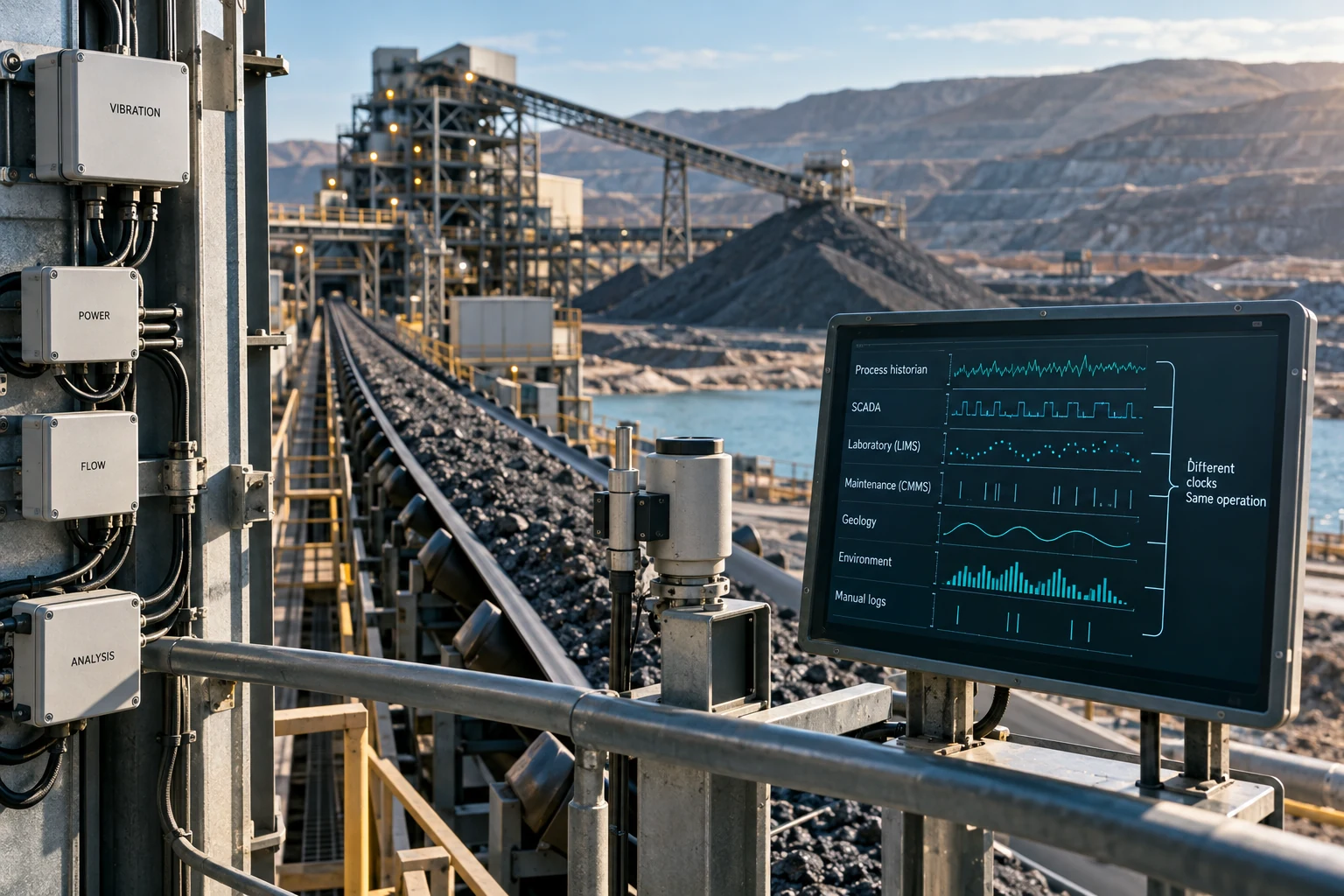
Our engineers start every mining or materials engagement with a written inventory of these systems: who owns the export, what the retention window is, and whether the archive is a faithful record or a compressed approximation. That document is often worth more to the customer than the model that follows it.

• Process historian. PI-class or Aspen IP.21 tag archives for the crusher, mill, flotation and dewatering circuits. Thousands to tens of thousands of tags.
• Fleet management. Position, payload, cycle states and engine telemetry off the SAE J1939 CAN bus for every truck, shovel and drill.
• Condition monitoring. Accelerometers, oil analysis, thermography and motor-current signatures on mills, crushers, gearboxes and conveyor drives.
• Laboratory system. Feed, concentrate and tails assays from the LIMS on a four- to twenty-four-hour turnaround, plus blast-hole assays.
• Geological model. Block model, grade-control polygons, drill logs and survey pickups, updated on a shift or daily cadence.
• Compliance monitoring. Dust and gas sampling, water discharge results, blast vibration, and the atmospheric monitoring system required underground by 30 CFR § 75.351.
• Maintenance system. Work orders, failure codes and close-out text. The only place ground-truth failures are recorded, and usually the messiest.
• Video and access. Fixed and vehicle-mounted cameras, badge records, and increasingly in-cab fatigue monitoring.

What that adds up to in volume

Volume decides where compute lives. A mid-size concentrator with 20,000 historian tags at one-second resolution generates about 1.7 billion values a day, though swinging-door compression of the kind PI applies by default usually shrinks the stored archive by an order of magnitude. That reduction is itself the problem, and we return to it below.

Vibration runs the other way. A triaxial accelerometer sampled at 25.6 kHz in 16-bit produces roughly 154 KB per second, or 13 GB per day from one sensor; fifty sensors streaming raw waveform would be about 240 TB a year. No mine ships that to a cloud, so features are extracted on the analyzer or a small edge box and only spectra and band energies travel. Video dominates everything else: one continuously recording 4K camera at 8 to 10 Mbps produces roughly 3 TB a month, and twenty of them are going nowhere on remote-site bandwidth. Fleet telemetry is trivial by comparison, a few megabytes per truck per day at 1 Hz. Set video aside, reduce vibration at the edge, and the genuinely modelable corpus at most sites is a few hundred gigabytes to a few terabytes a year. That is a laptop-scale problem wearing an industrial-scale costume.

Where the value is, in numbers

Metallurgical recovery is the biggest lever and the easiest to price. Take a copper concentrator treating 100,000 tonnes per day at a 0.5% head grade: 500 tonnes of contained copper a day. One percentage point of additional recovery is 5 tonnes per day, about 11,000 pounds. At $4.00 per pound and 350 operating days, that point is worth roughly $15 million a year. A model that reliably delivers a quarter of a point is still a multi-million-dollar result, which is why recovery projects survive budget review when dashboard projects do not.

Availability is second. On a 60-truck haul fleet, one percentage point of mechanical availability is six-tenths of a truck of hauling capacity with no capital spend. The same arithmetic applies to a main incline conveyor, where an unplanned belt failure stops the whole mine rather than one machine. Product quality is third and underrated: contracts price penalties on arsenic, moisture, ash or sulfur, and a model that predicts stockpile-blend chemistry a shift ahead pays for itself on penalties alone, using assay history that already sits in the LIMS.

Exposure is fourth by dollars and first by consequence. Continuous personal dust monitors, required in underground coal under 30 CFR § 70.201, produce a near-real-time record that pairs with ventilation, production and weather data. The useful output is a shift-level ranking of which crews and which faces are trending toward the limit, while there is still time to change the ventilation plan.

Four different clocks

These projects fail when a team builds for one latency budget and the customer needs another. There are four, and they call for four architectures.

Decision	Latency budget	Where it runs
Safety interlock, collision avoidance	10–250 ms	PLC or certified proximity hardware. Never a model.
Process setpoint advice	30 s – 5 min	Edge or on-prem server beside the historian and DCS.
Blend, grade and dispatch decisions	15 min – 8 h	On-prem or cloud, batch scored on a shift cadence.
Maintenance and reliability alerts	Hours to days	Cloud. Retraining weekly is generous.
Resource model and planning updates	Days to quarters	Cloud, with full lineage capture for disclosure.

Only the first tier drives hardware decisions. Everything below it tolerates a link that drops for an hour, so a remote site needs a store-and-forward buffer rather than premium connectivity.

The safety layer is not a place for a model

Proximity detection on continuous mining machines in underground coal is a regulated function under 30 CFR § 75.1732, and atmospheric monitoring systems are specified under 30 CFR § 75.351. Functions like these sit in certified hardware and rated logic assessed under IEC 61508 and IEC 61511. A statistical model has no defensible place inside that loop, and proposing one is a fast way to lose a mine's safety department.

Underground coal adds a second boundary. Electrical equipment used in gassy environments must be MSHA-approved as permissible under the explosion-proof and intrinsic-safety requirements of 30 CFR Part 18 and the approval procedures of 30 CFR Part 7. A general-purpose compute board cannot be carried inby and energized because someone wants better telemetry. In practice, models live in the advisory layer: they read from the historian and the AMS, they write to an operator display or a work-order queue, and they never actuate.

What the rest of the rulebook does to the architecture

Federal mine regulation is a data-generating machine, which is good news for anyone building here. Under section 103(a) of the Federal Mine Safety and Health Act of 1977, MSHA inspects every underground mine in its entirety at least four times a year and every surface mine at least twice, and every inspection, citation and reportable injury lands in a public dataset. MSHA's Mine Data Retrieval System publishes mines, inspections, violations, accidents and quarterly employment and production files, which makes external benchmarking possible without touching a customer's private data.

The same rules bound what a system may hold. Under 30 CFR § 50.10 an operator must notify MSHA within 15 minutes of knowing a reportable accident has occurred; injury records follow under Part 50, and MSHA may inspect and copy them under 30 CFR § 50.41. Training records under Part 46 for surface aggregate operations and Part 48 for underground mines are inspectable too. Anything a system records about an individual miner can reach an investigation file, so retention windows and access control are architecture requirements. Exposure limits set the accuracy bar: MSHA's 2024 respirable crystalline silica rule fixed a permissible exposure limit of 50 micrograms per cubic meter as an eight-hour time-weighted average with an action level of 25, phased by mine class, and underground metal and nonmetal diesel particulate matter is capped at 160 micrograms per cubic meter of total carbon under 30 CFR § 57.5060.

Disclosure, environment, and the audit trail

Anything touching resource or reserve estimation crosses into securities disclosure. SEC registrants report mining properties under Regulation S-K subpart 1300, codified at 17 CFR §§ 229.1300 through 229.1305, which replaced Industry Guide 7 for fiscal years beginning on or after January 1, 2021. Estimates must be supported by a qualified person and, for material properties, a technical report summary filed as Exhibit 96; Canadian and Australian issuers work under NI 43-101 and the JORC Code on the same logic. If a machine-learning grade estimate feeds anything a qualified person signs, the pipeline needs pinned data snapshots, versioned code, captured seeds and a written statement of assumptions defensible years later. We build that lineage in from the first commit, because retrofitting it after a model already influences a mine plan is expensive and sometimes impossible.

Environmental data is public and already structured. Effluent limitations for ore mining and dressing sit at 40 CFR Part 440 and coal mining at 40 CFR Part 434, and NPDES discharge monitoring reports are filed electronically under 40 CFR Part 127, so they surface in EPA's compliance database. Nonmetallic mineral processing carries air standards under 40 CFR Part 60 Subpart OOO, surface coal permitting and bonding run through the Surface Mining Control and Reclamation Act of 1977 and OSMRE's rules at 30 CFR Chapter VII, and hardrock work on public land runs under the General Mining Law of 1872 and BLM rules at 43 CFR Part 3809. Tailings monitoring is where spend has moved fastest since the Global Industry Standard on Tailings Management appeared in 2020: piezometer and inclinometer series, survey monuments, and satellite radar interferometry that measures millimeter-scale movement across a facility without a site visit.

The materials half of the problem

Materials work has the opposite data shape. Where a mine drowns in high-frequency readings with almost no labels, a materials program has rich labels and very few samples. A coating study or an alloy qualification campaign might hold 60 to 400 measured specimens, each expensive and each carrying real measurement uncertainty. Fitting a large model to 200 rows produces a confident number and no information.

What works is pairing computed data with measured data. Open density-functional-theory databases including the Materials Project, the Open Quantum Materials Database and AFLOW hold hundreds of thousands to millions of computed inorganic entries with formation energies, band gaps and elastic properties, all API-accessible. Those become features or pretraining targets, and the small experimental set becomes the calibration layer. The method is usually Gaussian-process or ensemble regression with honest uncertainty, driving a Bayesian optimization loop that proposes the next experiment. Federal demand is concrete: the Energy Act of 2020 directs USGS to maintain and update the critical minerals list, the 2022 list named 50 commodities, and USGS Mineral Commodity Summaries each January is a free external anchor for any model forecasting supply or substitution.

Why data quality decides the outcome

Model choice is close to irrelevant here. On tabular process data a well-tuned gradient-boosted tree and a well-tuned neural network land within noise of each other. Five unglamorous data problems separate a project that works from one that does not.

Compression deadbands. Historians store exceptions, not samples. Exception and compression deviation settings discard values inside a deadband, then draw a straight line between the survivors. Fine for a trend display, destructive for a model that depends on short-lived excursions. Read raw archive values where they exist, quantify how much of a tag is interpolated, and drop tags whose deadband is wider than the effect being modeled.

Clock skew. The DCS, the historian, the fleet system, the LIMS and the CMMS rarely share a time source, and a 90-second offset between two of them is common. A model reasoning about cause and effect on a five-minute process is then learning noise. The first engineering task is a clock audit against one event visible in every system, such as a mill trip.

Residence-time alignment. Ore takes 20 to 60 minutes to travel from the crusher through grinding to the flotation cells. Joining belt-scale grade to concentrate assay on a matching timestamp compares material that never met. Lag alignment, ideally with a variable lag estimated from throughput, is the highest-value transformation in a concentrator dataset, and it is arithmetic rather than machine learning.

Sampling error. Gy's theory of sampling, and the practice codified in ASTM D2234 for coal and ISO 12743 for concentrates, exists because a badly cut sample carries more error than any modeling choice can recover. If the cross-belt cutter is undersized or the riffle splitter is misused, the assay column is noise with a decimal point.

Gaps that are not random. Instruments go offline exactly when conditions get interesting, so the missing periods are the informative ones. Mean-imputing them teaches a model that upsets never happen. Missingness gets its own indicator feature and its own paragraph in the report.

Labels are the scarce resource

Failure prediction sounds like supervised learning and almost never is. A gearbox class across a whole fleet may fail three times in five years, which is three positive examples. Anomaly detection, survival methods and physics-informed residual models all beat a classifier at that sample size. The label source that does exist is the maintenance system, whose structured failure-code field is usually wrong because it is filled from a dropdown at the end of a long shift. The reliable signal is the free-text close-out narrative, and the correct workflow is model-assisted coding with a reliability engineer reviewing a sample rather than autonomous extraction.

False alarms carry a price that belongs on paper before the first model is fit. If a callout costs $800 in labor and inspection, and the system raises 40 alerts a month at 30% precision, the customer pays about $22,000 a month to chase 28 non-events. Set the operating threshold from that arithmetic, not from an F1 score.

What the bill actually looks like

Infrastructure is rarely the expensive part. Twenty terabytes in standard cloud object storage runs roughly $470 a month at $0.023 per gigabyte-month, with government regions somewhat higher. Egress surprises people: pulling that same 20 TB back out at $0.09 per gigabyte is about $1,800, which is the argument for processing where the data already sits. Training a gradient-boosted model on a few hundred million rows is one large-memory instance for a few hours, not a GPU cluster, and a ruggedized edge box at a motor control center is low four figures.

Engineering time is the real cost, and data access, alignment and validation dominate it. A scoped first engagement on one site and one asset class typically lands between $60,000 and $150,000 over eight to twelve weeks, fixed price. If a proposal puts most of that budget in the model and a slice in data engineering, the ratio is backwards and the project will overrun.

Scoping a first engagement that can fail cheaply

The best first project produces a defensible answer either way and ends on a date. Narrow it to one site, one asset class or circuit, one defined historical data cut, and one success metric agreed in writing before anyone sees a result.

Three details separate a cheap failure from an expensive one. Build the naive baseline before the model, because a rolling average or the existing alarm rule often lands within a few percent of the sophisticated answer, and that should surface in week six rather than month eighteen. Hold out a contiguous time block instead of a random split, since random splits leak across autocorrelated process data and inflate every score. And write the kill criterion into the statement of work, so ending the project is a normal outcome.

Common questions on the public-record framing

Bottom line

Mining and materials reward data engineering more than modeling. The instrumentation is installed, the regulatory record is public and structured, and the economics are unusually easy to price: a point of recovery, a point of availability, a penalty avoided. Projects fail at the join keys, the clock offsets and the sample cutters, long before anyone chooses an algorithm. A tightly scoped first engagement that pre-registers its metric, builds the baseline first and runs in shadow mode tells a buyer within a quarter whether the value is there.

Frequently asked questions