The alert nobody could spend against
Here is the pattern we get called into. A company instruments forty assets, trains models on eighteen months of historian data, and stands up a screen that flags degradation. The reliability engineer likes it. Six months later the program is quietly defunded. When you ask what went wrong, nobody says the model was wrong. They say some version of the same sentence: it told us a gearbox was degrading, and we already knew that, and it did not tell us whether to fund the rebuild in Q3 or wait for the outage in Q1.
That sentence is the whole problem. An alert says a signal moved. A capital decision needs a dated cash request, a consequence if the money is not spent, a confidence statement someone will sign, and a comparison against every other asset competing for the same pool. Programs that die are producing the first thing and being judged against the second.
The fix is not a better architecture. It is deciding, before any sensor is specified, which recurring decision the system exists to change. If the answer is the maintenance planner's weekly schedule, that is a legitimate and much cheaper system. If the answer is the capital plan, then the output format, the horizon, the uncertainty handling, and the validation evidence all change. Most programs are scoped as the first and judged as the second.
What separates a funded program from a defunded one — our weights
Weights sum to 100. Where we put engineering attention on a first build, from programs we have seen survive and not survive. Judgment, not measurement.
The horizon mismatch is the root cause
Vibration analytics detect bearing degradation weeks to months ahead. A capital plan is built nine to eighteen months ahead and locked at a specific date. Those two horizons do not touch. When a program produces two-week warnings and the planner needs twelve-month ones, every alert arrives as an unbudgeted emergency, which is exactly the cost the program was funded to eliminate.
The governing number is the P-F interval, the span between the moment an incipient failure becomes detectable and the moment the asset stops doing its job. It is asset-specific and it is knowable from your own failure history. Ask for it per asset class before agreeing to any sensor plan. If the P-F interval on a critical asset is three weeks, no model on earth turns that into a capital signal. That asset belongs in a condition-based work-order flow, not in the capital model.
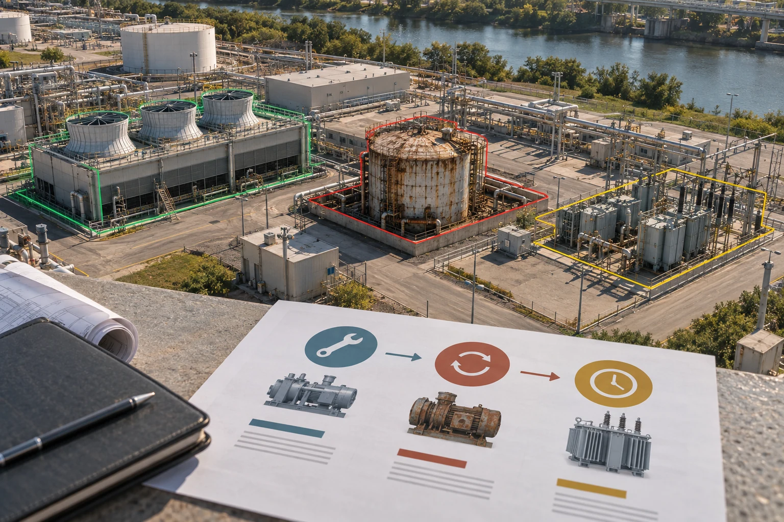
The assets that do belong in the capital model are the ones with long, slow, monotone degradation: large rotating equipment, transformers and switchgear, heat exchangers fouling, structural coatings, hydraulic power units, cooling towers. Their signals move over quarters. Those are the assets where a remaining-useful-life estimate can plausibly reach a planning cycle. Sorting your fleet into those two buckets on day one is the single highest-value hour in the project.
Remaining useful life is a distribution, not a date
A model that outputs "142 days" is unusable and, worse, it is dishonest. Physical degradation carries real uncertainty from load variation, operating context, sensor noise, and the fact that the specific failure mode has not yet declared itself. The honest output is a distribution: a median, a lower bound, and the probability the asset survives past a specific date that matters to the planner.
That last framing is what makes the output spendable. A planner does not need to know the mean life. They need to know the probability the asset makes it to the scheduled April outage. Recast that way, the model answers a question the budget process already asks, and the answer maps directly onto a decision: fund the rebuild in this cycle, defer to the outage, or accept the risk and hold spares.
Practically this means survival models rather than point regressors, or a point model wrapped in conformal prediction so the intervals carry a coverage guarantee under distribution shift. Weibull-based reliability models remain the workhorse for slow-degrading mechanical assets, with the advantage that reliability engineers already read them. Deep sequence models can beat them on richly instrumented assets, at higher validation cost and with less to say when someone asks why the number moved.
Price the deferral, not the failure
Most predictive maintenance business cases are built on avoided failure cost: multiply downtime hours by contribution margin per hour, subtract the program cost, present a payback. Controllers discount that arithmetic on sight, and they are right to. It assumes the failure was going to happen, assumes the model would have caught it, and assumes the plant would have acted. Three assumptions, none verified.
The number that survives scrutiny is the deferral value. For each candidate asset, the finance question is what it costs per week to keep running versus what it costs to intervene now. That is a calculation with observable inputs: the rebuild quote, the labor and crane cost, the outage window value, the spares carrying cost, and the escalating probability of an unplanned stop. Build that table per asset and the model stops being a science project and becomes an input to a decision the controller is already making.
There is a second number worth computing early, because it kills more programs than model error does. Every false alarm has a price: the planner's hours, the inspection labor, the teardown that finds nothing, and the credibility loss that makes the next alert ignored. Set the alarm threshold by minimizing total expected cost across missed detections and false alarms, using your own labor rates, rather than by maximizing an F1 score. Those two thresholds are rarely the same, and only one of them is defensible in a budget meeting.
| Asset class | Signal that carries the trend | Usable planning horizon | Belongs in |
|---|---|---|---|
| Large rotating equipment | Broadband vibration trend under ISO 20816, bearing defect frequencies, oil debris counts | Two to four quarters | Capital plan |
| Power transformers | Dissolved gas analysis ratios, moisture in oil, furan content, load history | One to five years | Capital plan |
| Heat exchangers | Fouling factor from thermal duty against clean baseline, pressure drop trend | One to three quarters | Capital plan |
| Medium-voltage motors | Partial discharge trend, motor current signature, insulation resistance and polarization index | Two to six quarters | Capital plan |
| Rolling-element bearings | Envelope demodulation, ultrasound, temperature | Weeks to a few months | Work-order flow |
| Hydraulic and pneumatic circuits | Cycle-time drift, actuator dwell growth, pressure decay | Days to weeks | Work-order flow |
Horizons are asset-specific and depend on duty. Establish yours from your own failure history before committing a sensor plan or a budget claim.
Your failure history is the constraint
The first hard conversation on any of these builds is about labels. A supervised remaining-life model needs runs that end in a failure, with a known failure mode and a known date. Most industrial fleets have five to fifteen such events per asset class in a decade, and many of them are recorded in a work-order free-text field as "replaced bearing" with no mode, no root cause, and a completion date that reflects when the paperwork closed rather than when the machine stopped.
Three things get built out of that. First, a failure-mode taxonomy for the fleet, usually anchored to ISO 14224 so the coding survives a change of contractor and can be compared against industry reliability data. Second, an extraction pass over historical work orders to recover mode and date from free text. Modern language models do this well and they do it wrong often enough that every extraction needs a reliability engineer sampling the output. Third, a censoring-aware training setup, because assets that were replaced on schedule and never failed carry real information and dropping them biases every estimate optimistic.
The data plumbing decides the schedule
The model is a small part of the calendar. Historian extraction, tag mapping, unit reconciliation, and operating-context joins take longer than everything downstream. Tags accumulate over twenty years with no naming convention, three tags for the same measurement at different scan rates, and a rename in 2017 that broke continuity on half the fleet.
Operating context is the piece that gets skipped and then wrecks the model. A vibration reading means nothing without load, speed, ambient temperature, and the product being run. A model trained across mixed context learns the context and calls it degradation. Pulling load and mode data out of the MES or ERP and aligning it to the sensor stream is where accuracy actually comes from.
On the interface side, data comes off through OPC UA under IEC 62541, Modbus TCP, or MQTT with Sparkplug B, crossing the Purdue-model boundaries of ISA-95 under the segmentation expectations of IEC 62443 and NIST SP 800-82 Rev. 3. Design the first system read-only, off a historian replica or a mirrored port. Controls engineers will not let a model write setpoints, and that is the correct answer. If any of the line touches federally funded work, check the equipment bill of materials against the covered-equipment restrictions in Section 889 of the FY2019 NDAA, implemented at FAR 52.204-25, before purchase orders go out.
Governance, because someone will ask
A model that moves capital is a model with financial consequence, and that pulls governance obligations that pure reliability work does not carry. For companies with a banking or insurance parent, SR 11-7 model risk management expectations reach any model whose output influences financial reporting or reserve decisions. For everyone else, the NIST AI Risk Management Framework is the reference text agencies and increasingly large primes cite, and ISO 42001 is the certifiable management-system analogue.
What that means concretely is modest and worth doing from the start. Document intended use and out-of-scope use, so nobody applies a compressor model to a pump. Record training data provenance and the operating envelope it covers. State performance by asset class rather than as a fleet-wide average, because a fleet average hides that the model is excellent on two hundred identical pumps and blind on the six critical assets. Keep a change log with dates and the responsible engineer. Establish who reviews a prediction before it becomes a funding request.
Where a first build's hours actually go — typical distribution
Distribution from builds of this shape. Yours shifts with historian quality and how well failures were coded.
Prove it backwards before you promise it forward
The only evidence that convinces a skeptical controller is a backtest on the company's own history. Freeze the model at a date two years back, run it forward on data it never saw, and show what it would have said before each failure that actually occurred. Then show the false alarms it would have raised in the same window, because a backtest that reports only the catches is marketing.
Structure that evaluation as a time-series split, never a random one. Random splits leak future information into training through neighboring samples from the same run and inflate every metric. Group by asset as well as by time, so the model is scored on machines it has never seen rather than on a second bearing from a pump it memorized.
Report three numbers to the business side. How many failures would have been caught with enough lead time to matter, using the P-F interval as the threshold for "enough." How many false alarms per hundred asset-months, at that same operating point. And the dollar difference between what was actually spent over that window and what the model's recommendations would have cost. The third number is the one that gets the program funded.
What a working system looks like in month six
The reliability engineer opens a ranked list each Monday. Each row is an asset, a failure mode, a probability of surviving to the next planned outage, the deferral cost per week, and a dated recommended action. The planner filters to the assets that will not make the outage and turns those into CMMS work orders without retyping anything.
Quarterly, the same model produces a different view for finance: the assets whose predicted intervention date falls inside the next planning cycle, sorted by deferral cost, totalled against the capital envelope. That view is one query against the same predictions, and it is the reason the program keeps its funding.
Underneath, a monitoring job watches for the thing that quietly kills these systems: input drift. A sensor gets replaced, a scan rate changes, the product mix shifts, and the model keeps producing confident numbers about a world that no longer exists. Population stability on the input features and a running comparison of predicted against realized failures catches it. Without that, the program is accurate for a year and wrong afterward, and nobody notices until the wrong call gets expensive.
Cost and time, honestly
For a scoped first build covering one plant and one to three asset classes, expect twelve to twenty weeks and a range of roughly $180,000 to $450,000 depending on historian condition, how many failure events exist, and whether sensor retrofit is in scope. Sensor retrofit itself is a separate line and usually larger than expected: on most retrofits the sensors are a minority of the installed cost, with conduit, cable tray, electricians, drawing updates, an outage to mount on a running asset, and historian tag licensing making up the rest.
The builds that come in low have a clean historian, a maintenance organization that codes failure modes, and a sponsor who named the decision before kickoff. The ones that run long are where the answer to which decision this changes arrived in week nine.
Bottom line
Predictive maintenance stops being a science project when its output is shaped like a funding request. That means a horizon matched to the planning cycle rather than the sensor rate, a probability of surviving to a specific dated outage rather than a point estimate, a deferral cost in dollars per week, an alarm threshold set by your own labor economics, and a backtest against your own failure history that shows the false alarms alongside the catches. Get those five right and the model can be ordinary. Get them wrong and no amount of accuracy will keep the program funded past its second budget cycle.
Frequently asked questions
For supervised remaining-life modeling on an asset class, roughly ten to thirty coded failure events is where estimates become defensible. Below that, start with anomaly detection against a healthy baseline plus physics-based degradation, and build the labeling discipline that makes the supervised version possible in two years.
Often yes, for a first pass. Historian tags already carry motor current, pressures, temperatures, flows, and cycle times, and those support fouling, leakage, and load-related degradation models. Bearing and gear diagnostics generally do need accelerometers mounted properly, because a magnet mount or handheld probe rolls off before the frequencies where early bearing energy lives.
Platforms handle ingestion, trending, and generic anomaly detection well. What they do not supply is your failure-mode taxonomy, your deferral economics, your operating-context joins, and the backtest against your own history. That work decides whether the output reaches a budget line, and it is specific to your fleet.
Under SR 11-7 expectations, a model influencing financial decisions needs documented intended use, independent validation, ongoing performance monitoring, and a named owner. NIST AI RMF and ISO 42001 cover the same ground for firms outside banking supervision. Two weeks of documentation during the build replaces a quarter of retrofit later.
Monitor input distributions for drift, compare predicted against realized failures on a rolling window, and re-validate whenever a sensor is replaced, a scan rate changes, or the product mix shifts. Those three events cause most silent failures in fielded maintenance models.