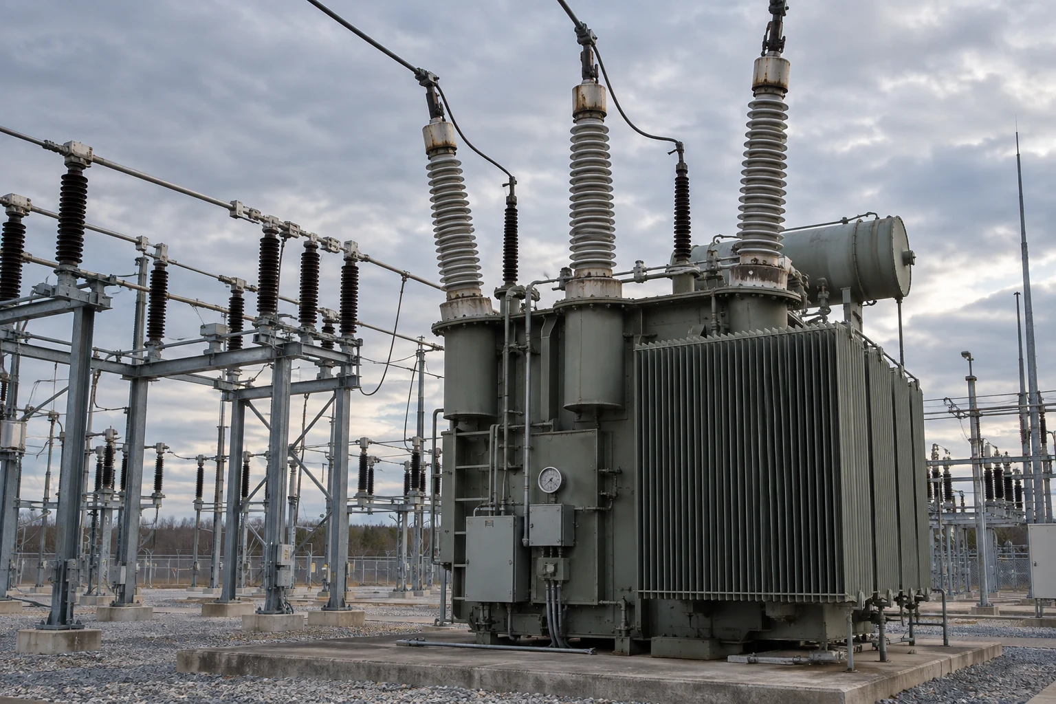
The data you actually get
Utility analytics efforts tend to begin with a diagram of a clean data lake and end in a room where somebody explains why the meter reads and the outage record disagree by four hours. Grid data comes out of systems built to control equipment and produce bills, and none of them were designed with a training set in mind. Anyone proposing work here should be able to name the source systems, the scan rates, the record volumes, and the regulatory zone each dataset sits in. That list is the statement of work.
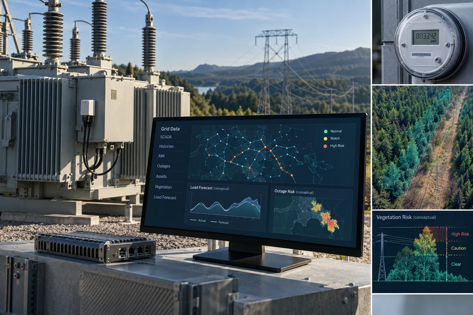
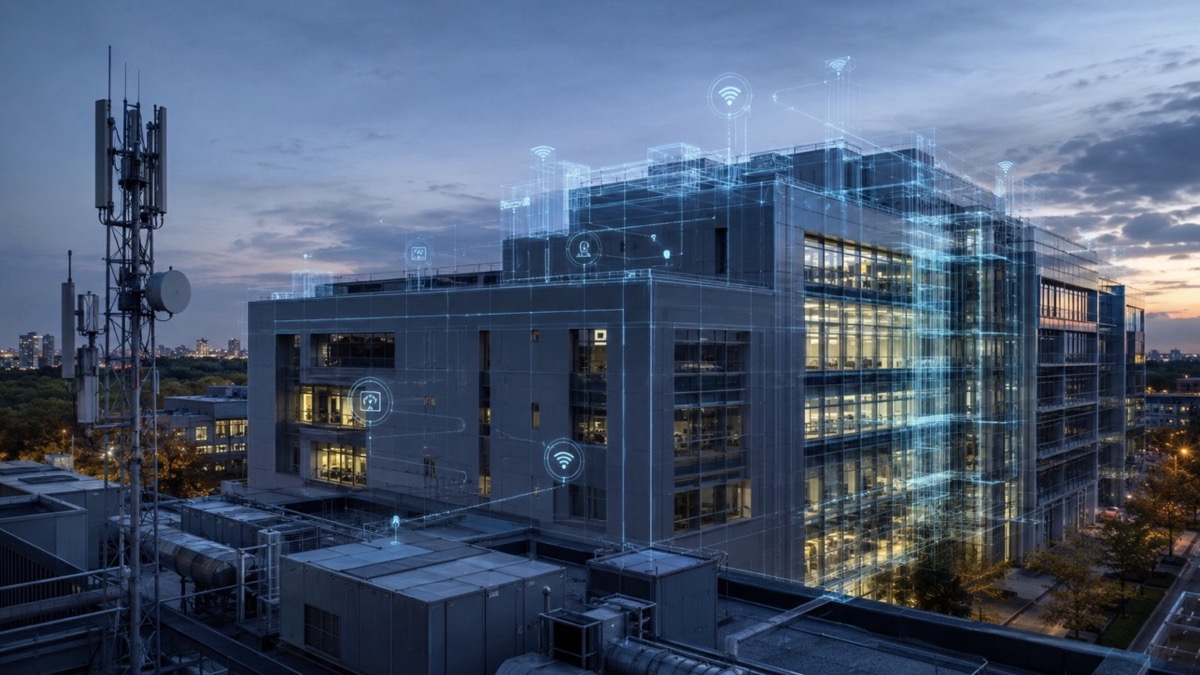
A typical investor-owned or federal utility holds the interesting data in six systems: the EMS and its SCADA front end, a process historian (usually OSIsoft PI or eDNA), the AMI head end and its meter data management system, an outage management system often fused with a DMS, a GIS carrying the connectivity model, and a work management system recording what crews actually did.
Each system has its own key for the same transformer. The GIS calls it a facility ID, work management calls it an equipment number, the historian calls it a tag path, and the nameplate carries a serial number that may or may not have been transcribed correctly in 1998. Reconciling those identifiers is not preparation for the modeling; on most grid programs it is the work, which is why we wrote separately about why grid asset data is a records problem first.
Utility AI use cases: value against feasibility on real data
Editorial weighting from public sources and practitioner reading. Illustrative, not a measured statistic.
SCADA, the historian, and what "real time" means
The EMS polls RTUs and intelligent electronic devices over DNP3 (IEEE 1815), IEC 61850 inside newer substations, and ICCP (IEC 60870-6, also called TASE.2) between control centers. Analog points are typically scanned every 2 to 10 seconds. Automatic generation control runs on a 2 to 4 second cycle, and the state estimator solves every 1 to 5 minutes. A mid-size EMS carries 50,000 to several hundred thousand points.
The historian is where analytics teams usually get access, and it is not a raw archive. Exception-based reporting and swinging-door compression store a value only when it moves outside a deadband, so the series is unevenly spaced and a naive resample fills the gaps with an interpolation the historian invented. Train on that and the model learns the compression settings. Quality flags matter for the same reason: a stale point still carries a plausible number.
Protection is not an analytics surface and should never be proposed as one. Relay decisions land in 4 to 16 milliseconds and IEC 61850 GOOSE messaging runs in the low single digits. Synchrophasors are different. PMUs stream at 30 or 60 frames per second under IEEE C37.118 and IEC/IEEE 60255-118-1, roughly 150 GB per year per unit, so a few hundred units puts a wide-area archive into the tens of terabytes a year. That archive earns its keep on oscillation detection and event forensics.
AMI is bigger than SCADA and worse behaved
Fifteen-minute intervals are the common AMI configuration: 96 reads per meter per day, 35,040 per meter-year. A million-meter territory generates about 96 million records a day and 35 billion a year on one channel, and utilities that also collect voltage, register reads, and event logs multiply that by three to six. Stored well this is not a capacity problem: columnar layout with delta encoding and ZSTD brings an interval value to a few bytes, so a million meters of 15-minute demand is on the order of 150 GB per year per channel.
The trouble is in the tail. Meters drop intervals during communication outages and backfill later. Clocks drift. A meter swap breaks the meter-to-premise mapping unless the CIS transaction lands cleanly. MDMS validation, estimation, and editing rules write estimated values that look measured except for a flag, and if that flag does not reach the training set, the model spends capacity learning the utility's own estimator.
Meter voltage is the most underused dataset in the stack. It supports phase identification, meter-to-transformer mapping, and detection of overloaded service transformers, and planning engineers use those outputs the day after delivery.
Outage prediction: the model is easy, the labels are hard
Two problems share this name. Storm outage prediction estimates how many interruptions will occur and where over the next 24 to 72 hours. Asset-driven prediction estimates which device is about to fail, and it hits the label scarcity described in the next section.
Weather features are the easy part. HRRR gives 3 km CONUS grids on hourly runs with an 18-hour horizon, extended to 48 hours on the 00, 06, 12, and 18Z cycles. Gust ratios, wind direction against line orientation, soil moisture, and leaf-on state carry most of the signal.
Labels are the hard part. They come from the OMS, where a dispatcher under storm load entered a predicted device, a restoration time, and a cause code. Cause code is usually the weakest column in the enterprise. Nested outages roll up to an upstream device, so one record can represent many faults. Honest evaluation reports IEEE Std 1366 metrics, notes whether a Major Event Day was declared under the 2.5 beta method, and separates major-event from blue-sky performance.
What makes this fundable is the decision it feeds. Crew staging and mutual assistance are committed 24 to 72 hours ahead of landfall, and those commitments cost real money. Predicting outage counts by operating district to within roughly a quarter of actual at 48 hours changes staging; a five percent gain on a system total changes nothing.
Asset condition: transformers first, then everything else
Power transformers get attention first because they are expensive, long-lead, and instrumented. Dissolved gas analysis is the workhorse. IEEE C57.104-2019 gives status levels for the combustible gases, and the Duval triangle maps gas ratios to fault types. Online DGA monitors sample hourly; offline lab samples come once or twice a year, and that interval is often the binding constraint on how early anything can be called.
The statistics are unforgiving. A fleet of 800 transmission transformers might produce a dozen genuine failures across ten years. That does not support a deep model, and a firm proposing one is telling the asset manager it has never worked the problem. What works is a survival or hazard formulation with physics constraints, explicit uncertainty, and calibration against the gas limits the engineers already trust.
The deliverable that gets funded is not a health index. It is a ranked capital and maintenance list with a dollar consequence on each line, because that is the one artifact an asset manager and a rate case can both use.
Vegetation management: the largest controllable outage driver
On transmission this is a compliance matter. NERC standard FAC-003 applies to applicable overhead lines at 200 kV and above, plus lines below 200 kV designated as elements of an Interconnection Reliability Operating Limit. It sets minimum vegetation clearance distances derived from the Gallet equation, and a sustained outage caused by vegetation inside the right-of-way is among the most serious findings a transmission owner can take. On distribution there is no NERC standard, and vegetation still drives a large share of interruption minutes.
Data arrives in layers. Aerial LiDAR at 20 to 40 points per square meter produces billions of returns and hundreds of gigabytes across a few thousand corridor miles in one flight season. Sentinel-2 multispectral imagery at 10 meter resolution on a five-day revisit gives growth rate and canopy change between flights.
The sequence is classification of ground, canopy, and conductor returns, then conductor position under thermal and wind loading, then growth projection by species and site, then a trim priority by span. The trap is temporal: most utilities fly a corridor once every three to five years, so the growth model carries the whole interval between captures.
Load forecasting: where the accuracy actually lives
Three horizons, three different problems. Very short term covers 5 minutes to 6 hours and supports dispatch and market position. Day-ahead covers 24 to 168 hours against a hard wall-clock deadline, because day-ahead energy markets in the eastern RTOs close in the late morning. Long-term forecasting produces peak demand and energy for planning studies and rate cases.
Observed accuracy sets the bar. Day-ahead system-level MAPE at a large balancing authority typically runs 1.5 to 3 percent, feeder-level forecasts run 5 to 15 percent, and a single service transformer only becomes tractable in aggregate. A proposal claiming feeder-level accuracy near the system-level number is either measuring something else or has leaked future information into the features.
Two regulatory changes reshaped the feature set. FERC Order No. 2222 opened RTO and ISO markets to distributed energy resource aggregations, so the forecast has to reason about resources the utility does not own and may not directly meter. FERC Order No. 881 made ambient-adjusted transmission line ratings a compliance requirement with an implementation deadline in July 2025, turning line ratings into their own forecasting problem. Behind-the-meter solar does the rest: a model trained on pre-solar years misses the afternoon net-load shape, and the fix is a separate PV disaggregation model.
NERC CIP decides where the data and the model may live
Section 215 of the Federal Power Act made NERC the Electric Reliability Organization and its Reliability Standards enforceable. Regional Entities audit against them, and statutory civil penalties run up to $1 million per violation per day. That is why a utility CIO declines an architecture that looks obviously correct to a cloud engineer.
CIP-002 categorizes BES Cyber Systems as high, medium, or low impact. Control centers, generation at or above 1,500 MW aggregate at one plant location in a single Interconnection, transmission facilities at 500 kV and above, and 200 kV to 499 kV stations above an aggregate weighted value of 3,000 land in the medium or high buckets, and that category drives every requirement that follows.
Those requirements shape analytics work directly. CIP-005 defines the Electronic Security Perimeter, bars direct routable connectivity into it, and forces Interactive Remote Access through an Intermediate System. CIP-007 sets a 35 calendar day cycle for evaluating security patches. CIP-010 requires a documented baseline configuration, change verification on at least a 35 day cadence, and scanning of transient cyber assets. CIP-013 puts vendor software under a supply chain risk management plan, CIP-015 adds internal network security monitoring, and CIP-008 requires notice of a Reportable Cyber Security Incident to the E-ISAC and CISA within one hour.
One revision matters to anyone designing a data platform. CIP-004-7 and CIP-011-3, effective January 1, 2024, restructured BES Cyber System Information so protection attaches to the information and its access controls rather than the storage location, which made third-party storage of BCSI workable under proper encryption and key management. That did not turn a real-time control application into a cloud application. A model that cannot be described to a compliance auditor in the same terms as the rest of the control system will not be allowed to run.
Three zones, three different answers
Inside a high or medium impact Electronic Security Perimeter: no external analytics platform, no outbound telemetry, change control under CIP-010. In the operations DMZ: read-only replication of historian and EMS data, one direction only. In the enterprise analytics zone: AMI, GIS, work management, customer and weather data, where normal cloud tooling is usually available once BCSI is kept out.
What an air-gapped or on-premises deployment changes
Utility OT networks follow the Purdue model, with the operations DMZ at level 3.5 mediating between control and enterprise. Where separation is strict, that mediation is a unidirectional gateway: data flows out, nothing flows in. That breaks the assumption underneath most commercial ML products, which expect a continuous loop of telemetry out and model updates back.
Everything downstream changes. No package manager during install, no model hub pull, no license check, no crash reporter. Every dependency is a signed artifact staged on media that passed a transient cyber asset scan. We covered what genuinely runs with zero egress in our piece on air-gapped inference; the failure mode is a library that quietly fetches something on first call.
Hardware is whatever the customer already has, and a substation rack is not a GPU cluster. Plan for CPU inference. A gradient-boosted model over 200 features scores a hundred thousand rows in under a second on one core, which covers forecasting, outage counts, and asset ranking. Language models are where the budget goes: an 8B model at int8 needs roughly 9 GB of memory, a 70B model at 4-bit about 40 GB and a real accelerator.
Evaluation becomes a local artifact: the test suite ships with the model, writes metrics to files the customer can open, and reports drift without calling home. Retraining runs on the quarterly rhythm the change process can absorb, so the model has to degrade gracefully when inputs shift.
| Data source | Typical volume | Latency the decision needs | Usual zone |
|---|---|---|---|
| EMS / SCADA points | 50K–500K points, 2–10 s scan | Seconds to minutes | Inside the ESP |
| Process historian | Years of compressed tag history | Minutes to hours | Replica in the DMZ |
| Synchrophasor (PMU) | 30–60 frames/s, ~150 GB/yr per unit | Sub-second to minutes | Inside the ESP |
| AMI interval data | 96 reads/meter/day, ~35B rows/yr per million meters | Hours to a day | Enterprise analytics |
| OMS / DMS events | Thousands of events per storm | Minutes during an event | Operations, replicated out |
| GIS + work management | Millions of asset and work records | Days | Enterprise analytics |
Who is buying this work
The federal side is larger than most software firms realize. Bonneville, Western Area, Southwestern, and Southeastern are power marketing administrations under the Department of Energy. The Tennessee Valley Authority runs a full generation and transmission system, and the Bureau of Reclamation and the Army Corps of Engineers own much of the hydro behind that power. These are NERC-registered utilities with the same CIP obligations and the same aging asset records, and they buy through federal contract vehicles.
Infrastructure Investment and Jobs Act money, including the Grid Resilience and Innovation Partnerships program and the section 40101(d) state formula grants, moves through state energy offices to municipal utilities and cooperatives that have the data and not the staff. Investor-owned utilities usually buy through incumbent engineering and IT primes, which makes subcontract scope the normal entry point. Precision Federal builds AI, data, and software systems for federal, state, and commercial customers, as a prime and as a subcontractor.
A 90-day path that produces something a utility will use
Programs stall when they try to model everything at once. The engineers we assign to this work start from the zone map, pick one decision, and reconcile only the records that decision touches.
First 90 days on a grid data engagement
Bottom line
Value concentrates in forecasting tied to a real deadline, storm decisions made 24 to 72 hours ahead, and asset spending ranked against consequence. Risk concentrates in where the data and the model may live. Treat the CIP boundary as an architecture input and the system ships; treat it as paperwork and it stays a pilot.
Frequently asked questions
It depends on whether the data qualifies as BES Cyber System Information. CIP-004-7 and CIP-011-3, effective January 1, 2024, made third-party storage of BCSI workable when access controls and key management protect the information itself. The determination is made per dataset with the utility's CIP compliance group, before any pipeline is built.
At the common 15-minute interval, 96 reads per meter per day and 35,040 per meter-year. A million-meter utility generates roughly 35 billion records a year on one channel, compressing to about 150 GB per year in a columnar store. Voltage, register, and event channels multiply that several times over.
Day-ahead MAPE at the balancing-authority level typically runs 1.5 to 3 percent. Feeder-level forecasts run 5 to 15 percent depending on customer mix and behind-the-meter solar. Individual service transformers are only forecastable in aggregate.
CIP applies to the Bulk Electric System, so purely distribution assets generally fall outside it, and CIP-002 categorization is the test. Utilities outside CIP scope still face state commission requirements, IEC 62443 practice for OT security, and customer data obligations.
Nearly all of the high-value work. Gradient-boosted models, probabilistic forecasters, survival models for asset risk, and point-cloud pipelines run acceptably on CPU. GPUs become necessary for language models and heavy imagery.