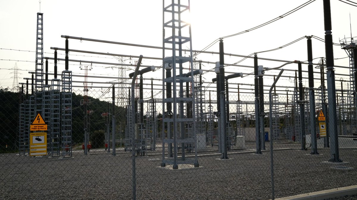
Four forecasts, one name
When someone says the load forecast is bad, the first job is to find out which forecast they mean. A utility runs at least four, they answer to different people, they are wrong in different ways, and improving one does nothing for the others. Buying a model before separating them is how a project ends up with a beautiful day-ahead curve delivered to a planning group that needed a ten-year peak.

| Horizon | Decision it feeds | Who lives with it | What accuracy actually means here |
|---|---|---|---|
| Very short term Minutes to a few hours | Dispatch, switching, reserve posture | The control room | Ramp shape and turning points, not level |
| Day ahead Hourly, next one to seven days | Purchases, schedules, unit commitment | Power supply and scheduling | Hourly error where prices are highest, not the daily mean |
| Peak alerting Which hour tops the month | Curtailment calls, demand response, load shifting | Whoever owns the wholesale bill | Did you call the right hour. Everything else is noise |
| Long term Annual peaks, five to twenty years | Capacity, capital plan, rate case support | Planning and finance | Whether the growth assumptions are defensible in writing |
A large system's day-ahead hourly forecast typically lands somewhere in the range of one and a half to three percent mean absolute percentage error. A single substation or feeder is a different animal entirely, commonly five to fifteen percent, because diversity is what makes aggregate load smooth and a feeder has very little of it. One irrigation district, one plastics plant, one data hall, and the feeder stops resembling a curve and starts resembling a switch. Anyone who quotes you a system-level number for a feeder-level product is not being careful.
You are probably here because
- The wholesale bill jumped and it traces to two afternoons in July
- The forecast that scored well all year missed the week that mattered
- Afternoon load stopped behaving the way it did five years ago and nobody rebuilt the model
- Planning and operations quote different peak numbers in the same meeting
All four point at the same thing: the forecast is being scored on the average and paid for on the extremes.
The peak hours are the entire bill
For many distribution utilities and cooperatives, a large share of annual wholesale cost is set by demand in a small number of coincident peak hours. Whether it is one hour a month or a handful of hours a year depends on your contract, but the structure is nearly always the same: an enormous amount of money riding on a tiny number of intervals. A forecast that is excellent on the other eight thousand hours and misses those has not helped.
This should change what you build. The product is not a curve. It is a call. Somebody has to decide, usually the afternoon before, whether tomorrow is a peak day and whether to spend real money reducing load: notifying interruptible customers, running distributed generation, shifting pumping, pre-cooling. Each call has a cost when it is wrong in either direction. Calling a peak that does not arrive burns goodwill with the customers who curtailed, and there are only so many times a year you can ask. Missing a peak sets a demand charge you carry for twelve months.
So the forecast should output a probability that a given day contains the monthly peak, and it should be scored against the decision, not against megawatts. Ask your current vendor a simple question: over the last three years, how many of the actual peak hours did the forecast rank in its top three candidates for that month? That number is worth more than any error statistic, and most programs have never computed it.
Weather is most of the signal and you do not control it
On a hot-summer system, temperature and humidity explain the overwhelming majority of day-ahead variance. Which means your forecast error is mostly inherited weather forecast error, and no amount of modelling skill recovers it. If tomorrow's high is off by three degrees, your load will be off, and the honest ceiling on your accuracy is set by your weather provider rather than by your algorithm.
Practical consequences. Buy more than one weather feed and score them against each other on your own service territory rather than on national skill scores, because vendors differ locally and the local difference is the only one you pay for. Use the spread across providers as an uncertainty signal: when three forecasts disagree by four degrees on Thursday, the load forecast for Thursday deserves a wider band and a human should see it. And use the right variables. Dry-bulb temperature alone is a weak proxy for cooling load; humidity matters, and building thermal mass means the previous two days matter too. A model with lagged and smoothed temperature terms usually beats one with today's high, and that gap is larger than most algorithm choices.
Weather stations are their own small trap. A station that moved, a sensor that drifted, or a gap that your provider silently interpolated will show up as an unexplained model error weeks later. Keep the raw observations and record which station each reading came from.
Behind-the-meter solar broke the old temperature curve
Load used to rise monotonically with afternoon temperature, which made the modelling comfortable. On systems with meaningful rooftop solar, what the utility sees is net load, and net load falls in the middle of the day and then climbs steeply as output drops through the late afternoon. The peak migrates later. The steep evening ramp becomes the operationally interesting part of the day. And cloud cover becomes a first-class input, because a cloudy hot day and a clear hot day now have different shapes rather than different levels.
Two things follow. First, if your training data spans the period in which local solar adoption doubled, the relationship you are fitting is not stable and the model will systematically misread recent years. Either model gross load and subtract an estimated solar production series, or include an installed-capacity term that lets the fit move. Second, you probably do not know your installed capacity accurately. Interconnection records lag, and small systems get missed. Estimating aggregate behind-the-meter output from clear-sky irradiance and a capacity estimate, then reconciling against observed midday net load, is unglamorous work that produces more improvement than any change of algorithm.
Where day-ahead error comes from — a summer-peaking system, our decomposition
Illustrative decomposition for a summer-peaking system with visible rooftop solar. Yours will differ; the last row is usually the smallest and gets the most attention.
Meter data arrives late, and then it changes
Interval meter data is the best input a utility has and the most misunderstood. Reads arrive over hours to days, some meters miss a communication window and backfill later, and the validation and estimation process substitutes values for gaps and then revises them. A read you pulled on Tuesday is not necessarily the read that will be in the system on Friday.
This ruins a model quietly. If training rows are built from settled, fully revised data and the production model runs on whatever arrived by six in the evening, you have trained on information the model will never have. The result is a system that validates beautifully and underperforms in service, and the gap is often larger than any modelling improvement you were chasing.
The fix is to store data with two timestamps: when the interval occurred, and when you learned the value. Then build training rows using only what was known at the equivalent hour on that historical day. It is more work than reading a table, and it is the difference between a number you can trust and a number you cannot. The same discipline applies to estimated versus actual reads, which should never be silently interchangeable, and to meter changes, which produce a discontinuity that looks exactly like a behaviour change.
A backcast on observed weather is not a forecast
The single most common way a load model is oversold is by evaluating it with the weather that actually happened rather than the weather that was forecast at the time. This removes the largest error source in the problem, and it is not unusual for it to make a model look roughly twice as accurate as it will be in service. Insist on evaluation against archived weather forecasts, at the same lead time the production system will use. If your vendor cannot supply archived forecasts, that is itself an answer.
We will score your current forecast honestly, for free.
Send two years of hourly actuals, the matching forecasts your system produced at the time, and your peak-hour definition to contact@precisionfederal.com. You get back the error broken out by hour of day, by temperature band, and by whether the day contained a peak — plus how often the peak hour was ranked correctly. One business day.
contact@precisionfederal.comThe scheduler who overrides the model is telling you something
Every utility has someone who adjusts the forecast before it is used. Often they have done it for twenty years, often the adjustment is right, and often the modelling team treats it as an insult. It is not. It is a free labelled dataset about what the model does not know.
Log every override: the hour, the direction, the size, and one sentence on why. Within a season you will have a list of the model's blind spots in the operator's own words, and they are usually specific and fixable. The county fair. The plant that runs a Saturday shift in harvest season. The first genuinely cold morning of the autumn, when heating load behaves differently than it does at the same temperature in February. Most of those become features. A few become a note in the interface saying the model has no information about this, which is also a useful thing for the interface to say.
Do not remove the override. A forecast a control room cannot adjust is a forecast a control room will stop opening, and you will hear about that when it is far too late.
What we would not build
- A single model for every horizon. Dispatch and capital planning need different inputs and different owners
- A deep network on three years of hourly data when gradient-boosted trees with proper weather features are within noise and can be explained
- A point forecast with no band for a decision that is fundamentally about risk
- Customer-level forecasts when nobody has named a decision that changes because of them
- A retraining job that pulls whatever is in the meter table today, mixing revised and unrevised reads without noticing
- An accuracy dashboard that reports the annual average and nothing about peak hours
And a case for doing nothing at all. If you buy power under a fixed all-in rate with no demand component and no market exposure, better accuracy has almost no dollar value to you, and the correct answer is to leave the forecast alone and spend the money on something that does. We have said this to utilities that were expecting a proposal. Ask what a one percent improvement is worth in your contract before anyone builds anything; if nobody can answer, that is the first piece of work.
What a first build looks like
Ten weeks, in the order we would do it
Step three frequently ends the project in the best possible way. Sometimes the incumbent forecast is already good, the peak-hour ranking is already strong, and the honest recommendation is to keep it and spend the budget on the meter data foundation instead. That is a cheap answer to have bought.
Step six matters more than it looks. A forecast earns its way into operational use by being visibly right for a season while nothing depends on it. Cutting the parallel run to save six weeks is how a good model gets switched off after one bad Tuesday, because nobody had built any reason to trust it yet.
Before you commission anything
- You know which of the four forecasts the project is for
- Someone has stated in dollars what an accuracy gain is worth in your contract
- Evaluation uses archived weather forecasts at production lead time
- Error is reported separately for peak days and peak hours
- Training data respects when each value became known
- Estimated and actual meter reads are distinguishable everywhere
- Behind-the-meter solar is modelled explicitly, not absorbed into a trend
- The output carries a band, and the peak-day call carries a probability
- Operator overrides are logged with a reason and reviewed each season
Bottom line
Load forecasting rewards care about inputs far more than cleverness about models. The gains that are actually available sit in weather feed selection and local scoring, in modelling distributed solar rather than letting it corrupt a temperature relationship, in reconstructing history so the model trains on what was knowable, and in reporting error where the money is instead of where it is convenient. Aim the product at the decision: for most utilities that decision is which afternoon to act on, not what the curve looks like on an ordinary Tuesday in April.
Frequently asked questions
At system level on a large service territory, roughly one and a half to three percent mean absolute percentage error is the usual range, with worse performance on extreme days and holidays. Individual feeders and substations are much harder, commonly five to fifteen percent, because they lack the diversity that smooths an aggregate. Treat any single quoted figure as meaningless until you know the aggregation level, the horizon, and whether it was measured against forecast weather.
Usually a little, and much less than the marketing suggests. Gradient-boosted trees on well-constructed weather and calendar features tend to beat a classical regression by a modest margin and are hard to beat further without adding data rather than model capacity. The larger gains almost always come from better weather inputs, explicit treatment of distributed solar, and honest handling of late-arriving meter data. Model choice is real but it is not where the headroom is.
Three to five years of hourly load with matching weather is a reasonable working minimum, mainly so the model has seen several summers and several cold snaps. More history helps only if the system it describes still exists. If your territory added substantial rooftop solar, electric vehicle charging or a large new customer during that window, older years describe a different system and should be weighted or corrected rather than trusted.
It can rank candidates well and it cannot be certain, which is why the output should be a probability rather than a call. The practical measure is how often the actual peak hour appeared in the model's top few candidates for that month, evaluated over several years. That number is directly comparable to what your team achieves today and is the only accuracy statistic that maps onto the decision you actually make.
You need more than one source and a record of how each performs on your own territory, which is not the same as buying a premium feed. Score the providers you can get against your own stations for a season, use the disagreement between them as an uncertainty signal, and keep the raw observations so a moved station or a drifting sensor can be found later rather than showing up as unexplained model error.