
The unit of cost is a GPU-hour
Nobody's serving stack is billed per token. It is billed per accelerator per hour, whether you rent by the hour, reserve for a year, or buy the hardware and amortise it. Your cost per token is that hourly number divided by the tokens you got out of the hour, so every serving decision you will ever make is a fight over the denominator. Once you see it that way the whole subject gets simpler, and the places where teams lose money become obvious.

Write it once and keep it on a wall:
cost per million output tokens = (hourly rate per accelerator × accelerators in the replica × 1,000,000) ÷ (output tokens per second × 3,600)
An eight-accelerator node at a blended twelve dollars an hour, sustaining a thousand output tokens per second across all concurrent requests, costs about three dollars and thirty cents per million output tokens. Push the same node to three thousand tokens per second and the number falls to a bit over a dollar. Nothing about the model changed. The denominator changed, and the denominator is set by batching, which is set by memory.
Two caveats before the arithmetic, and both matter more than they look. Hourly rates move constantly and vary by a factor of three or more between an on-demand hyperscaler instance, a specialist provider, a long reservation and depreciated hardware you own. Any number in this article is an illustration for the method, not a quote. And utilization sits outside the formula entirely, which is why it is the last section and the one that most often decides the answer.
You are probably here because
- Someone asked whether hosting the model yourselves would be cheaper and nobody could answer with a number
- Your inference bill grew faster than usage and the finance team noticed
- You have accelerators reserved and no idea what fraction of them is doing work
- A long-context feature shipped and throughput fell off a cliff nobody predicted
All four are answered by the same cost model. Build it once, in a spreadsheet, from measured throughput rather than a vendor benchmark.
Decode is bound by memory bandwidth, not compute
This is the fact that explains most of what feels counter-intuitive about serving costs, and it is worth internalising precisely.
Generating one output token for one sequence requires reading every weight the model uses for that token out of high-bandwidth memory and into the compute units. The arithmetic done with those weights is trivial by comparison — roughly two floating-point operations per parameter. Modern accelerators can do far more arithmetic per byte moved than that ratio requires, so the memory system is the bottleneck and the compute units sit partly idle.
Work an example. A seventy-billion-parameter dense model at sixteen-bit precision occupies about 140 GB of weights. On an accelerator class delivering roughly 3.3 terabytes per second of memory bandwidth, reading those weights once takes about 42 milliseconds. If you generate for a single sequence, that is your floor: about 24 tokens per second, and no amount of extra compute helps. Split the model across eight such accelerators with tensor parallelism and each holds an eighth of the weights, so the read time drops toward five milliseconds per token, minus real communication overhead that eats a meaningful share of the gain.
Now batch. Read those same weights once and use them for sixty-four sequences simultaneously. The memory traffic is unchanged; the token output is sixty-four times higher. This is the single largest lever in inference economics and it is why an idle model is so much more expensive per token than a busy one. Continuous batching — where finished sequences leave the batch and new ones join mid-flight rather than waiting for the whole batch to complete — is table stakes in every serious serving engine for exactly this reason.
Prefill is the other regime. Processing the input prompt is compute-bound, because you process all input positions in parallel and there is real arithmetic to do. Prefill scales roughly with total input tokens; the attention component scales worse than linearly with sequence length. This is why a workload with long inputs and short outputs behaves nothing like a workload with short inputs and long outputs, and why one throughput number for your service is usually a lie. Measure and report the two separately.
The KV cache is what actually limits your batch size
If batching is the lever, the key-value cache is the thing that stops you pulling it. Every sequence in flight holds a cache of the attention keys and values for every token it has seen, on the accelerator, for the whole life of the request. That memory competes directly with the weights.
The size is computable: 2 × layers × key-value heads × head dimension × bytes per element × sequence length. For a large model with eighty layers, eight key-value heads after grouped-query attention, a head dimension of 128 and sixteen-bit storage, that is roughly 320 KB per thousand tokens of context per sequence. A sequence at 8,000 tokens holds about 2.6 GB. At 128,000 tokens it holds about 41 GB — on its own, a substantial fraction of a single accelerator's memory.
Two consequences follow, and both surprise people.
Long context is the most expensive product decision in your stack. Moving a feature from an 8,000-token window to 128,000 does not cost you sixteen times more in prefill alone. It collapses your maximum concurrent batch by a similar factor, which raises the per-token cost of every other request sharing the node. Teams ship the long-context feature, watch throughput fall, and go looking for a bug. There is no bug.
Grouped-query attention is worth more than it sounds. Reducing the number of distinct key-value heads — sharing them across query heads — cuts cache size by that same ratio, commonly a factor of four to eight in current architectures. That factor converts directly into batch size, and batch size converts directly into cost per token. When you compare two models of similar quality, their attention configuration may matter more to your bill than their parameter count.
| Where a serving dollar goes | Typical share | What moves it |
|---|---|---|
| Accelerator time, decode | 50–70% | Batch size, quantization, model size, output length |
| Accelerator time, prefill | 15–35% | Input length, prefix caching, chunked prefill scheduling |
| Idle and headroom capacity | 10–40% | Traffic shape, autoscaling floor, cold-start time, redundancy |
| Host, network, storage, egress | 3–8% | Weight loading, checkpoint storage, cross-zone traffic |
| Engineering and on-call | Often the largest single line | Number of models, number of regions, release cadence |
The shares overlap because they trade against each other and because workload shape swings them hard. The row worth staring at is the last one: it does not appear on the accelerator invoice, and on small and mid-size deployments it is routinely bigger than everything above it combined.
What actually moves cost per token — our ranking of the levers
Our ranking from deployments we have costed, not a benchmark. The last row is where teams start and the first is where the money is.
Utilization is the multiplier that dwarfs the rest
Everything above assumes the hardware is busy. It usually is not, and this is where the difference between a spreadsheet and an invoice comes from.
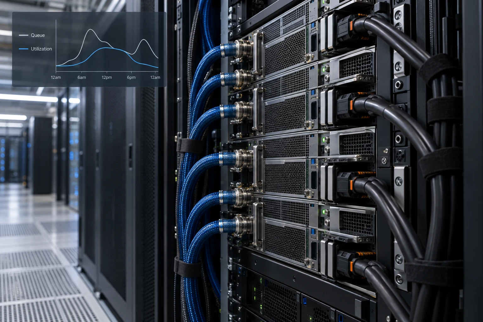
An interactive product used during working hours in one or two time zones has a demand curve with a peak-to-average ratio commonly between three and six. Size for the peak and you own idle capacity for most of the day. If you provision for peak and your average utilization lands at twenty percent, your effective cost per token is five times whatever the saturated arithmetic said. That single factor overwhelms every optimisation in the ranking above.
This is also the honest answer to why a hosted inference API can charge you less than your own hardware costs. They are not doing magic with kernels. They are aggregating thousands of uncorrelated demand curves into one much flatter curve, filling the troughs with batch work, and selling at a rate that assumes utilization you cannot reach alone. You are, in effect, buying someone else's statistical smoothing.
Cold start is why you cannot simply autoscale the problem away. Bringing a new replica up means scheduling a node, pulling a container, loading tens or hundreds of gigabytes of weights into accelerator memory, and warming the runtime. Several minutes is normal; ten is not unusual on a cold image. Traffic that arrives in twenty seconds cannot be served by capacity that takes five minutes to exist, so you either hold warm headroom — which is idle cost by another name — or you shed and queue.
The three-tier shape is what usually works. Own or reserve the base load where the discount for commitment is largest. Rent on demand for the predictable daily peak. Have a documented shedding and queueing policy for the tail, because buying capacity for a spike you see twice a quarter is the most expensive insurance in the stack.
Measure throughput at your latency target, never at peak
Every serving engine will happily report a throughput number achieved at a batch size that pushes time-per-output-token past anything a person will sit through. That number is real and useless. Fix your latency target first — time to first token and time per output token, at p95, on your actual prompt distribution — then find the largest batch that holds it. That is the throughput to divide by. Costing from a peak-throughput benchmark is the most common way a self-hosting business case comes out wrong by a factor of two or more.
Send us your traffic shape and we will build the cost model with you.
Email your request volume by hour, your input and output token distributions and your latency target to contact@precisionfederal.com. You get back a written estimate of cost per million tokens under rent and under host, the utilization assumption each depends on, and which one we would choose. One business day. No charge, no meeting, no deck.
contact@precisionfederal.comThe costs that never appear on the accelerator invoice
Self-hosting is an engineering commitment, not a procurement one, and the business case is usually decided here rather than in the token arithmetic.
People. A serving stack that is actually on-call — upgrades, capacity, incidents, model rotations, kernel and driver regressions — is a standing responsibility for two to four engineers who could be building product instead. Price them at your loaded cost and put the number in the same table as the hardware. On many deployments it is the largest line by a wide margin, and leaving it out is the single most common reason a self-hosting case looks better on paper than it turns out to be.
Redundancy. One replica is a demo. Production means at least two, in at least two failure domains, each sized to carry the load if the other is gone. That is not a ten percent uplift, it is closer to a doubling of the floor.
Evaluation and rollout. Every model change, quantization change, engine upgrade and kernel update needs a run against your eval suite before it reaches users. That compute is real, it is recurring, and it should be budgeted as a fixed monthly line rather than discovered.
Storage and movement. Weights are big. Multiple versions, multiple regions, pulled repeatedly by autoscaling replicas. It is not a large share of the total, but cross-zone and cross-region traffic on a chatty deployment surprises people, and it is entirely avoidable with local caching.
The second model. Nobody stays on one. A router, a small classifier, an embedding model, a judge for evaluation. Each is another set of weights competing for memory, another deployment to keep current, and another entry in the on-call rotation.
Where the rent-versus-host line actually sits
There is no universal threshold, but there is a reliable way to find yours, and the shape of the answer is consistent across the cases we have costed.
Rent when volume is low or spiky, the workload is interactive with a sharp daily curve, you want frontier-level quality, or your team is small enough that two engineers on serving is two engineers not on product. Most companies are here, and being here is not a failure of ambition.
Host when you have steady round-the-clock load that keeps hardware genuinely busy, a smaller or tuned model whose quality you have already validated against the task, a hard requirement that data stay inside your own boundary, or a workload that is batch and latency-tolerant enough to fill the troughs.
The middle is where money is lost. Moderate volume, interactive traffic, a frontier-class model, and a reserved fleet sitting at fifteen percent utilization. The rented equivalent would have cost less and freed the engineers. If your projected utilization is below roughly forty percent sustained, the arithmetic almost never favours hosting, and the arithmetic gets worse when you include the payroll line.
What to measure, and what to publish internally
Output tokens per second per accelerator, at your p95 latency target. Not peak. Not the vendor's figure. Yours, on your prompt distribution, under your batching policy. This is the denominator and everything else is derived from it.
Sustained utilization over a full week. Not a peak-hour snapshot. The Sunday-night number is part of your cost.
Cost per successful task, not per token. An agent that retries three times costs three times as much and produces one result. A cheaper model that needs two passes is not cheaper. Report cost against the unit the business actually cares about, joined to the outcome, or you will cut cost and quality at the same moment and see only half of it.
Cost by feature and by tenant. Tag every request. Without the tag you cannot tell which feature is expensive, which customer is unprofitable, or whether last month's increase was growth or a regression. Adding the tag later means backfilling from logs that do not have it.
The mistakes we get called in to fix
- A business case built on peak throughput at a batch size no user would tolerate
- Reserved capacity sized for peak, running near twenty percent average, with nothing filling the troughs
- Long context enabled everywhere, collapsing batch size for every request on the node
- No payroll line in the comparison, so hosting won on a spreadsheet that omitted its largest cost
- Untagged requests, making cost per feature and cost per tenant permanently unknowable
- Autoscaling with a five-minute cold start against traffic that arrives in twenty seconds
- Quantization shipped without an eval run, trading a quality regression nobody measured for a cost saving somebody did
- One replica in one zone, described in the plan as production
A two-week costing exercise
Serving Cost Model
Step three is the one worth insisting on. Every published benchmark uses a prompt distribution that is not yours, and the difference between a synthetic 512-token prompt and your real 6,000-token one is not a correction factor, it is a different regime. Replay your own captured traffic or the number is decoration.
Before you commit to hardware
- Throughput measured on your own traffic at a written p95 latency target
- KV cache per sequence computed for every context length you offer
- Sustained weekly utilization estimated honestly, including nights and weekends
- Redundancy priced as a second full replica in a second failure domain
- Two to four engineers costed into the hosted case at loaded rate
- Cold-start time measured, and the autoscaling policy checked against it
- Quality validated after quantization, on the same eval suite, before it counts as a saving
- Every request tagged by feature and tenant from the first day
- Cost reported per successful task, not per token
- The break-even volume written down, with the date you will re-check it
Bottom line
Serving cost is one division: accelerator-hours over tokens produced. The numerator is a market price you mostly cannot change. The denominator is memory bandwidth divided among however many sequences you can fit in the cache, multiplied by the fraction of the day your hardware is doing anything at all. Batching and utilization are worth more than every kernel-level optimisation combined, and the payroll line is worth more than both on most deployments. Build the model in a spreadsheet with your own measured numbers, put the engineers in it, and the rent-or-host answer will usually be obvious — often uncomfortably so.
Frequently asked questions
Because the API provider aggregates many uncorrelated demand curves and runs at a utilization you cannot reach with one workload. Your hardware costs the same per hour whether it is saturated or idle, and a typical interactive product leaves it idle most of the day. Add redundancy and two to four engineers on call and the gap widens further.
Memory. The weights occupy a fixed amount and every in-flight sequence holds a key-value cache proportional to its context length. Concurrency is roughly the leftover memory divided by cache-per-sequence, which is why long context is expensive far beyond its prefill cost — it shrinks the batch for everything else sharing the node.
Usually yes, and by more than the memory saving suggests, because smaller weights mean less traffic across the memory bus on every decode step and more room for KV cache and therefore a larger batch. The caveat is quality: run your full eval suite before and after, and treat an unmeasured quality regression as an unpaid cost rather than a saving.
Volume alone is the wrong question; sustained utilization is the right one. If you can keep hardware busy well above roughly forty percent across a full week — usually meaning round-the-clock or batch-heavy load — hosting starts to compete. Below that, the idle hours plus the engineering commitment generally make renting cheaper even at large token counts.
Cost per successful task, tagged by feature and tenant. Cost per token hides retries, multi-step calls and abandoned sessions, all of which multiply the real figure. Joining spend to outcome is also what stops a cost reduction that quietly traded away quality from looking like a win.