Model monitoring in practice: catching drift before a user does

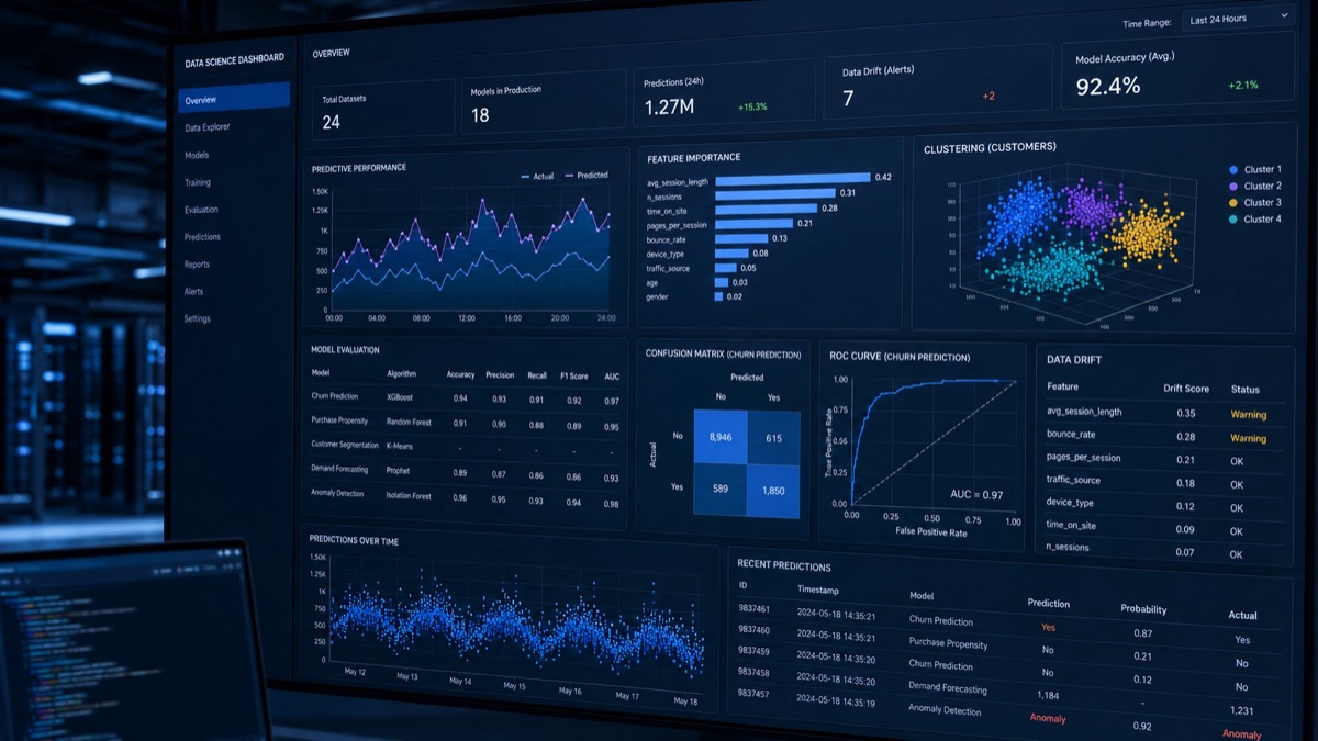
What model monitoring actually covers

The dangerous failure is the silent one. The service returns 200, the latency graph is flat, the uptime dashboard is green, and the predictions have been sliding away from reality for six weeks. Nothing alerts, because nothing broke in the way alerting tools understand. The first person to notice is a user or an auditor, and by the time that happens the trust cost is already paid and cannot be refunded by a fast fix.

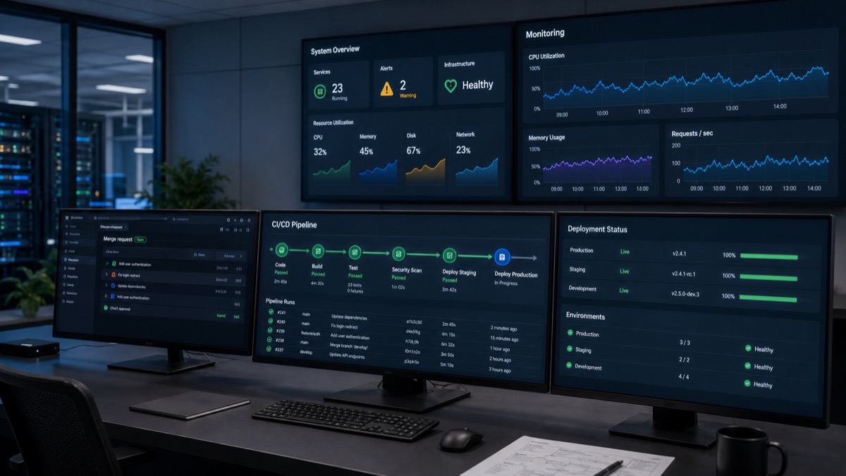
The word "monitoring" gets stretched across four jobs that need four different mechanisms. Infrastructure health asks whether the service is up and fast. Data health asks whether the inputs still look like what the model was trained on. Model behavior asks whether the predictions are distributed the way they used to be. Outcome quality asks whether the predictions are right. Standard observability tooling covers the first job well and the other three not at all. Teams that assume otherwise ship models with no real coverage, then discover the gap during an incident review.

The split that governs every design decision here is between signals you can compute immediately and signals you have to wait for. Input checks are immediate. Prediction-distribution checks are immediate. Accuracy is not, because accuracy needs labels, and labels arrive on the organization's schedule rather than the model's. A fraud score can wait up to 120 days for a card-network chargeback to confirm or refute it. A benefits eligibility recommendation may not be tested until an appeal is filed, and under 20 CFR 404.909 a claimant has 60 days to request reconsideration. A maintenance prediction is settled when the part fails or does not. Nearly every hard tradeoff in monitoring design comes from that lag.

The four things that break

Naming the failure classes separately matters, because each one has a different signal, a different detection latency, and a different fix. Treating them as one undifferentiated "drift" problem is how teams end up with a dashboard nobody can act on.

• Upstream pipeline breakage A join changes, a source system renames a column, a nightly load runs late and the model scores on stale rows. Fastest to detect, most common in practice, and usually the largest single source of bad predictions.
• Data drift The input distribution moves. New geography, new product mix, a policy change that shifts who shows up in the queue. The model is still doing what it was trained to do on a population it was not trained on.
• Concept drift The relationship between inputs and outcome changes while the inputs look unchanged. Fraud tactics adapt. A regulation changes what counts as a valid claim. This is the hardest class to see without labels.
• Training and serving skew The feature computed at scoring time differs from the one computed at training time. Different code path, different time window, different null handling. The offline metrics were never achievable in production.
• Model staleness Nothing broke. The world simply moved far enough from the training snapshot that performance decayed gradually. Only visible against a long baseline.
• Feedback loops The model's own outputs change the data it later sees. A queue ranked by risk score gets reviewed in score order, so labels only exist for high scores, and the next training set inherits the bias.

The decisions that are expensive to reverse

Most of monitoring is cheap to change later. Four things are not, and all four are schema decisions made in the first week.

Log the feature vector as scored, not the raw request. If the prediction log stores only the incoming payload and features are recomputed later for analysis, then every investigation is run against a different pipeline than the one that served the prediction. Training and serving skew hides in exactly that gap, and it becomes invisible to the tool meant to find it. Storing the resolved feature vector alongside the prediction is the single highest-value row in the schema. Add it in month nine and every incident before that date is unanalyzable.

Stamp versions on every row. Model version, feature-pipeline version, and code commit. When a metric steps on a Tuesday, the first question is what deployed that Tuesday. Without version stamps that question takes a day of archaeology; with them it takes one query. This costs a few bytes per prediction and pays for itself the first time it is needed.

Choose the join key to outcomes before launch. Every accuracy metric depends on connecting a prediction to what actually happened. If the outcome lands in a separate system under a different identifier, the join has to be reconstructed later from timestamps and fuzzy matches, which is expensive and unauditable. Agreeing on a stable key with the system of record is a one-hour conversation that saves a quarter.

Freeze a reference window and keep it. Drift is always measured against something. If the reference is a rolling trailing window, slow drift is invisible by construction, because the baseline moves with the data. Our practice is to hold a frozen training-period reference for absolute comparison and a rolling window for change detection, and to report both. Retiring the frozen reference later means losing the ability to answer how far the system has moved since the model was accredited.

What "good" means, numerically

Monitoring gets treated as unmeasurable, which is odd, because it is a detection system and detection systems have precision and recall like anything else. Four numbers are worth writing into the design document before any code is written.

Detection latency, per failure class. Pipeline breakage should be caught within one batch cycle. If the model scores nightly, that means the next morning at the latest. Distribution shift large enough to matter should surface within three to seven days. Performance decay is bounded by label arrival and cannot be faster than the label cycle, which is why proxy signals carry the load in between.

Alert precision. The share of pages that correspond to something a person should act on. A monitoring system whose alerts are right half the time is healthy. Below about thirty percent, the on-call rotation stops reading them, and at that point the system has negative value because it also provides false assurance. Our bar is that anything permitted to page a human clears fifty percent, and everything else opens a ticket or lands on a weekly review.

Coverage. The fraction of predictions that are logged with a complete feature vector and version stamps. Sampled logging is a reasonable cost decision at high volume, but the sampling rate has to be recorded, because every confidence interval computed downstream depends on it.

The noise floor. This is the number teams skip, and skipping it is why so many drift dashboards cry wolf. Metrics on finite samples move on their own. Score 1,000 items a day against a true error rate of five percent and the binomial standard error is the square root of 0.05 times 0.95 over 1,000, about 0.69 percentage points. Two standard errors is roughly 1.4 points. A daily error rate that wanders between 3.6 and 6.4 percent has told you nothing at all. Any threshold set tighter than the noise floor generates pure false alarms, forever.

Drift statistics and what their thresholds mean

Every drift tool ships with a default statistic and a default threshold, and the defaults are usually presented without the assumptions that make them reasonable. The table below is the short version of what our engineers use and where each choice misleads.

Statistic	What it measures	Where it works	Where it misleads
Population Stability Index	Binned distribution shift against a reference	The workhorse. Convention from credit scoring: under 0.10 stable, 0.10 to 0.25 moderate, above 0.25 significant	Fully dependent on binning. Ten bins and twenty bins give different answers on the same data
Two-sample Kolmogorov-Smirnov	Maximum gap between two cumulative distributions	Continuous features, no binning needed	At large n it flags shifts too small to affect any prediction. Significance is not importance
Chi-square	Categorical frequency change	Category mix, discrete codes, low-cardinality fields	Breaks down on rare categories and on new category values that did not exist in the reference
Jensen-Shannon divergence	Symmetric, bounded distributional distance	Comparable across features because it is bounded on a fixed scale	Still needs binning for continuous inputs, and the threshold is domain-specific rather than universal
Wasserstein distance	Cost of moving one distribution onto another	Respects magnitude, so a shift of two units reads larger than a shift of one	Scale-dependent, so it needs normalization before features can be compared to each other
Classifier two-sample test	Can a model tell reference rows from current rows	Catches multivariate drift that per-feature tests miss entirely	Heavier to run and to explain. An AUC near 0.5 is the healthy result, which reads backwards on a dashboard

One habit is worth adopting regardless of statistic: weight drift by feature importance. A large shift in a feature that barely affects the prediction is a curiosity. A small shift in the top feature is an incident. Ranking the drift table by importance times magnitude cuts the review queue sharply without losing what matters.

The label-delay problem

If labels arrived instantly, monitoring would be a solved problem: track accuracy, alert on a drop, retrain. They do not arrive instantly, and the interval between prediction and truth is where the design work lives.

The first move is proxy signals that correlate with performance and need no labels. Prediction distribution is the strongest of these. If a risk model that has flagged four percent of cases every week for a year suddenly flags nine percent, something changed, and it changed before any label could tell you. Score histograms, mean predicted probability, and the rate of predictions near the decision boundary all move early. Confidence calibration on the subset that does have labels, even a small subset, extends the signal further.

The second move is a deliberate labeled sample. Rather than waiting for organic outcomes, route a small random slice of predictions to human review on a fixed cadence. Two hundred reviewed items a week gives a usable read on precision within a few points, arrives on a known schedule, and does not suffer the selection bias that plagues organic labels. On systems where a reviewer already touches the output, this costs almost nothing beyond the instrumentation to sample randomly rather than by score.

The third move is to record predictions in a form that supports backfilled evaluation. When labels finally land, the evaluation should reconstruct exactly what the model saw on the day it scored, including version and feature values. That is the payoff for the schema decisions above.

How monitoring goes wrong

Multiple comparisons. Test 200 features every day at a 0.05 significance level and roughly ten will trip by chance daily, fifty a week, none of them real. The fix is standard statistics applied consistently: control the false discovery rate with a Benjamini-Hochberg procedure, or set thresholds on effect size instead of p-values, or both. Teams that skip this step build an alert stream with a floor of noise that never goes away.

Aggregate metrics hiding segment collapse. Overall accuracy holding at ninety percent is consistent with one segment at ninety-six and another at sixty-one. If the small segment is the one that matters legally or operationally, the top-line number is actively misleading. Segment the metrics along the dimensions where a failure would be consequential, and set thresholds per segment, accepting that small segments have wider noise bands and need correspondingly looser bounds.

Static thresholds against seasonal data. Volume, mix, and outcome rates in most federal and commercial workloads have weekly and annual structure. A fixed threshold set in March will fire every December. Either compare against the same period in prior cycles or model the seasonality explicitly before differencing.

Alert fatigue as a design outcome. Every alert that pages a human and turns out to be nothing raises the odds the next real one gets dismissed. Alert precision is not a nice-to-have metric; it is the mechanism by which the entire system retains value. Tiering matters here: page for pipeline breakage and hard schema violations, ticket for sustained distribution shift, and put slow trends on a weekly review that a person actually reads.

Production concerns: latency, cost, and the on-call bill

Monitoring belongs off the critical path. Cheap inline checks are fine, and a schema and range validation on the input costs microseconds and prevents a category of garbage-in failures outright. Everything heavier goes asynchronous: write the prediction record to a queue or an append-only store and compute statistics in batch. A synchronous call to a monitoring service inside the request path adds its tail latency to the p99 of the model and creates a dependency where an outage in the observability stack takes down the service being observed.

Storage is usually smaller than teams fear and query is usually larger. Ten million predictions a day at two kilobytes of feature vector and metadata is twenty gigabytes a day, about 600 gigabytes a month. At roughly $0.023 per gigabyte-month for S3 Standard in commercial regions, with government regions priced higher, the raw retention bill is modest. The cost that grows is repeated full scans by a dashboard that recomputes everything on every page load. Partition by date and model version, precompute daily aggregates once, and let the dashboard read summaries. That one change routinely cuts the observability bill by an order of magnitude.

The largest real cost is human. A monitoring system generates work: triage, investigation, decisions about whether to retrain. Budget it honestly. A model with meaningful consequence needs a named owner and a standing weekly review of an hour, plus whatever incidents cost. A build with no assigned reader produces dashboards that go stale within two months.

The federal overlay

Federal deployments add requirements that make monitoring a compliance artifact rather than an engineering nicety. OMB Memorandum M-25-21, issued April 3, 2025 and replacing M-24-10, requires agencies to apply minimum risk-management practices to high-impact AI, including pre-deployment testing, an impact assessment, ongoing monitoring after deployment, and human oversight. A model in that category needs monitoring evidence that can be handed to a reviewer, not a Grafana board an engineer can narrate.

The NIST AI Risk Management Framework, AI 100-1, puts the same expectation in its MANAGE function, where MANAGE 4.1 calls for post-deployment monitoring plans that are implemented rather than merely written, with mechanisms for capturing user input, appeal and override, and decommissioning. For the security side, NIST SP 800-53 Rev. 5 supplies the control language that assessors already know: CA-7 for continuous monitoring, SI-4 for system monitoring, AU-6 for audit review and analysis. Mapping the model monitors onto those control identifiers, in the System Security Plan, is what turns an engineering practice into an accreditation artifact.

Two operational details follow. Prediction logs frequently contain controlled unclassified information, which pulls the monitoring store into the same protection scope as the model itself under NIST SP 800-171 and, on DoD contracts, DFARS 252.204-7012, including the 72-hour cyber incident reporting obligation to DIBNet. A monitoring database standing outside the authorization boundary is a finding waiting to happen. And on FedRAMP-authorized services, continuous monitoring already has a defined rhythm of monthly vulnerability scans and POA&M updates, with a significant-change request required before material modifications. A retraining pipeline that swaps model weights automatically should be reviewed against the significant-change process before it is switched on, not after.

Monitoring the monitor

The quietest failure in this whole area is a monitoring job that stops running. The dashboard keeps showing the last computed values, everything looks stable, and stability is exactly the symptom. Every monitoring pipeline needs a heartbeat: an alert that fires when the expected computation has not completed within its window. Freshness of the monitoring output is itself a monitored metric.

The companion practice is backtesting monitors against known incidents. Replay a past outage or data-quality event through the current configuration and check whether it would have fired, how fast, and at what tier. A monitor that would not have caught the last real incident is not yet tuned. The exercise takes an afternoon and routinely finds intuition-set thresholds off by a factor of several.

When a simpler method is the right answer

Not every model justifies a monitoring platform. A model scoring 500 items a day, feeding a human who reviews every output, with a decision that is reversible, needs a weekly sample of thirty cases checked by hand and a chart of daily volume. That is honest coverage for that risk level, it costs an hour a week, and it will surface real problems faster than a drift dashboard nobody opens.

Three rules of thumb hold up. If a human reviews every prediction before it takes effect, the human is the monitor and the instrumentation only needs to make their disagreements countable. If the model runs monthly, monitoring can run monthly, and continuous streaming infrastructure is a cost with no matching benefit. If the input source is a single controlled internal system with a stable schema, freshness and row-count checks catch most of what will ever go wrong, and per-feature statistical testing adds noise more than insight.

The inverse is worth stating plainly. Automated retraining is the piece teams reach for first and should adopt last. A trigger wired to a drift metric can chase noise into a worse model with no human in the loop to notice. Earn that automation after the monitoring has proven trustworthy for a few cycles.

Bottom line

Model monitoring is a detection problem, and it responds to the same discipline as any other detection problem: name the failure classes, pick a signal for each, set thresholds above the noise floor, measure alert precision, and give the output to a person whose job includes reading it. The schema decisions made in week one determine what can ever be investigated, so make those deliberately. Everything else can be tuned as the system teaches you what normal looks like.

Common questions on scope and rigor

Frequently asked questions