
Classify before you model
The first mistake is applying one method to four thousand items. Demand series come in kinds, the kinds respond to different treatment, and telling them apart takes two numbers you can compute from history in an afternoon.
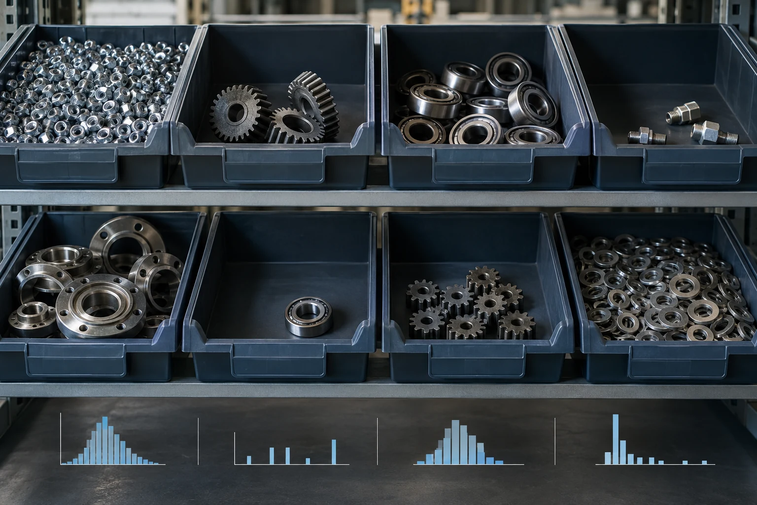
The first is the average interval between demands — how many periods pass, on average, between orders. The second is the variability of the order sizes when demand does occur, usually expressed as the squared coefficient of variation. The literature on intermittent demand uses cut points near an interval of 1.32 periods and a squared coefficient of variation near 0.49 to split series into four groups: smooth, intermittent, erratic and lumpy. Treat those cut points as useful conventions from the published work rather than as laws of nature; what matters is that you separate the groups at all.
Work an example. A part sold four times last year, in quantities of 40, 120, 15 and 300. The average interval between demands is about thirteen weeks. The mean order size is 118.75, the standard deviation of those four sizes is about 112, so the coefficient of variation is about 0.94 and its square about 0.88. Long gaps and highly variable sizes: that is the lumpy corner, and it is the hardest one. Its annual total is 475 units, which is knowable and plannable. Its weekly average of 9.1 is a number that has never once been ordered.

You are probably here because
- The system forecast is a fraction of a unit and the planners override all of it
- You are simultaneously stocked out and sitting on dead inventory
- A vendor promised a large accuracy improvement on items that sell four times a year
- Service level is a target nobody can trace to a stocking decision
The section on forecasting the distribution instead of the mean is the reframe that makes the rest work. The section on known demand is where most of the real improvement usually comes from.
The reframe: you do not need a point forecast
For a lumpy item, the mean is arithmetically correct and operationally meaningless, because the decision is not “how much will sell next week.” The decision is how much to hold so that when an order does arrive, you can fill it at the service level you promised, given how long replenishment takes.
That decision needs a distribution of demand over the replenishment lead time, and a quantile of it. If lead time is six weeks and you want to cover the great majority of arrivals, what you need is the upper tail of “how much could be ordered in any six-week window,” not the average of the weekly series.
Once you frame it that way, several things resolve. Fractional forecasts stop being embarrassing, because you never look at them directly. The service level target becomes a quantile choice with a visible inventory cost. And the whole question moves from “how accurate is the forecast” to “how much stock buys how much service,” which is the trade the business is actually making.
Methods that fit the shape
The classical approach separates the two things that vary. Rather than smoothing demand per period, smooth the size of demand when it occurs and the interval between occurrences, then combine them. That is Croston's method, published in 1972, and it remains the sensible starting point.
Two refinements are worth knowing. Croston's estimator carries a known bias, and the Syntetos–Boylan approximation applies a correction for it. And the Teunter–Syntetos–Babai method updates the probability that demand occurs in every period rather than only when it does, which makes it react more sensibly to an item that has gone quiet — a real advantage in a catalog full of parts drifting toward obsolescence.
The pragmatic alternative, and frequently the best one, is to skip parametric estimation and resample history directly: draw lead-time windows from the observed record, many times, and read the quantile you need off the resulting empirical distribution. Bootstrap approaches of this kind are well established for intermittent lead-time demand. They make no distributional assumption, they handle a series of mostly zeros with occasional spikes without special cases, and their output is exactly the object you need.
They also have an honest limit worth stating: a bootstrap can only produce sizes it has seen. If your history contains no order above 300, the resampled distribution will not contain one either, and a new customer with a bigger appetite is outside its range by construction. Where that risk is real, blend in judgment rather than pretending the history covers it.
Accuracy metrics that lie to you here
Percentage error metrics fail on series with zeros. The mean absolute percentage error divides by the actual value, so it is undefined in every zero period and enormous in small ones. Applied to intermittent data it produces numbers that look like measurements and behave like nonsense.
Worse, optimizing against them selects a specific bad model. Forecasting nearly zero every period scores well on several error statistics for a series that is nearly always zero, and it will never tell you to stock anything. The model that wins the accuracy comparison is the one that guarantees the stockout.
Use a scaled error measure — the mean absolute scaled error is the standard choice and is defined in the presence of zeros. Then, more importantly, evaluate against the decision. Simulate the policy over held-out history: given this method, how much inventory would we have held, and what fill rate would we have achieved? Two methods land as two points on an inventory-versus-service plot, and the comparison is immediately meaningful to the person who has to fund the stock.
| Series type | What it looks like | Reasonable treatment |
|---|---|---|
| Smooth | Demand most periods, stable sizes | Ordinary exponential smoothing or a seasonal model; this part is not hard |
| Intermittent | Gaps between orders, consistent sizes | Croston family; the interval is the thing being estimated |
| Erratic | Orders most periods, wildly variable sizes | Model the size distribution; look for the one customer driving it |
| Lumpy | Long gaps and variable sizes | Bootstrap the lead-time distribution; expect judgment to matter |
| Known | Open orders, contracts, customer releases | Not a forecasting problem at all — capture it and stop modeling it |
The forecast that beats every model
In industrial businesses, a large share of what looks like random demand is not random. It is known to somebody in the building and is not in the planning system.
Open orders and backlog. Blanket purchase orders with releases against them. Customer planning releases arriving by EDI, which many customers already send and which frequently land in an inbox rather than in a planning table. Contract minimums. Project timelines a customer discussed with a salesperson in March. A maintenance overhaul at a customer plant that will generate a spares order in the same quarter it generates one every three years.
The single largest improvement available to most companies with lumpy demand is not a better statistical method. It is capturing the demand information that already exists, attaching it to the right item, and letting the statistical model handle only the genuinely unknown remainder. It is unglamorous work — parsing releases, connecting a customer's forecast to your part numbers, giving sales a place to record a known project — and it moves the number more than any model change we have seen.
The corollary matters too. Once known demand is captured, do not double-count it. The statistical forecast should cover the residual, not the whole, or you will build inventory for orders you already have on the books.
Demand is not shipments
Almost every company trains on shipment history, which records what was sold rather than what was wanted. When an item was out of stock, the demand does not appear at all — the customer bought elsewhere, substituted, or waited without telling you. Train on that and you learn your own constraint, then reproduce it, then confirm it.
The correction is a data capture change rather than a modeling one. Record the event when a customer asks for something you cannot supply: the item, the quantity, the date, and whether they substituted. Most order entry systems have somewhere to put this, and most companies do not use it. A year of that record is worth more than a change of algorithm.
Substitution is the related trap. If two parts are interchangeable and the counter staff pick whichever is on the shelf, then the two series are one series wearing two names, and forecasting them separately will over-stock both. Ask the counter, not the data.
Aggregate to where the signal is
A series that is unforecastable at the item-customer-day level is often quite regular at the family-site-month level. Long gaps are an artifact of slicing thinly: a part ordered four times a year is a mostly-zero weekly series and a perfectly ordinary annual number.
So forecast where the pattern is visible and push the result down using recent proportions, or forecast at the item level and roll it up, and reconcile the two so the planning numbers and the financial numbers do not diverge. Both directions are legitimate; what is not legitimate is having a plant total and a sum of item forecasts that disagree and no rule for which one wins.
Two practical notes. Aggregating over time — weekly to monthly — is often the cheapest useful change, because a monthly bucket may contain enough demand to model while the weekly one does not. And a review cycle finer than the replenishment lead time is mostly ceremony; if it takes six weeks to get material, a weekly re-forecast changes very little of what you can actually do.
Turning the distribution into a stocking decision
The textbook safety stock formula assumes demand is roughly normal. Lumpy demand is not remotely normal — it is a mass of zeros with a long right tail — so the formula understates the stock needed for a high service level and, on some items, overstates it for a modest one. Neither error is visible from inside the formula.
Use the empirical or bootstrapped lead-time distribution instead and read the quantile that matches your service target. It is less elegant and it is right for the shape of the data you actually have.
Then include lead time as a random variable, because it is one. Supplier performance varies, and a plan built on the average lead time is a plan that fails in exactly the periods when it matters. Sampling both demand and lead time when you build the distribution is a small amount of additional work and it is where a large share of real stockouts is hiding.
Finally, be specific about what “service level” means. The probability of not stocking out during a cycle and the fraction of demand filled from stock are different quantities, and on lumpy items they diverge sharply — one large unfilled order barely moves the first and badly damages the second. Pick the one your customers actually experience, and state which you are targeting.
Backtesting without fooling yourself
Time series demand a specific discipline: hold out the most recent periods, fit only on what came before, and roll the origin forward so you evaluate many forecast dates rather than one lucky one. Random train-test splits leak the future into the past and produce results that will not repeat.
Then hold the comparison to a real baseline. On intermittent items the honest baselines are a naive one — the same period last year, or a moving average of recent demand — and, more importantly, what your planners currently do, including their overrides. A method that cannot beat the incumbent process is not an improvement no matter how modern it is, and planners frequently know things the data does not contain.
Where you do not need us
If nobody has yet plotted a histogram of order sizes for the top hundred items, do that first. It takes an afternoon, it will identify the items where one customer is the entire series, and it often changes the plan before any modeling begins.
If your planning parameters were set from an export several years ago, refreshing minimum and maximum levels from the actual recent lead-time distribution is two weeks of work and will beat a new model on most catalogs.
If your planners override everything the system produces, adding a better model changes nothing until you find out why. Sit with them for a day. Frequently they are compensating for something structural — a lead time that is wrong in the master data, a customer whose releases never reach the system — and that is the fix.
Where outside help earns its keep is the segmented build: classifying the catalog, running different methods per segment, capturing known demand from documents and messages, simulating policy over held-out history, and wiring the chosen quantiles back into the planning system. That is a matter of a few months, and the largest share of it is data plumbing rather than modeling.
The mistakes that repeat
- One method for the entire catalog, when the catalog contains four different kinds of series
- Judging models by percentage error, which is undefined on zeros and rewards forecasting nothing
- Training on shipments and thereby learning your own stockouts
- Ignoring known orders that are already sitting in an inbox or a contract
- Double counting known demand after finally capturing it
- Normal-distribution safety stock on a series that is mostly zeros
- Treating lead time as a constant when supplier variability is where the stockouts live
- Re-forecasting weekly on items with a six-week replenishment lead time
- Reporting a forecast accuracy gain instead of an inventory and service position
A sequence that works
- Classify every item by demand interval and size variability before choosing any method
- Capture known demand first — open orders, releases, contracts, named projects
- Record unmet demand so the history stops being a record of your own constraint
- Forecast the lead-time distribution, not the weekly mean, for anything lumpy
- Sample lead time as a variable alongside demand
- Evaluate by simulated policy — inventory held against fill rate achieved
- Backtest with a rolling origin, and beat the planners' current process or stop
- Set the review cycle to the replenishment lead time rather than to the calendar
Bottom line
Lumpy demand is not a failure of forecasting; it is a different problem wearing forecasting's clothes. Split the catalog into kinds, accept that for the lumpy kind the useful output is a distribution over the lead time rather than a number per week, and choose the stocking quantile deliberately with its cost visible. Then do the unglamorous half, which is usually the bigger half: capture the orders you already know about, start recording the demand you could not fill, and check whether your lead times in the master data resemble reality. Judge all of it by inventory held against service delivered. If someone offers you a large forecast accuracy improvement on items that sell four times a year, ask which metric — the answer will tell you a great deal.
Frequently asked questions
Start by classifying rather than choosing. For genuinely lumpy items, the most practical approach is to resample history into lead-time windows and read the quantile you need from the empirical distribution, because it makes no distributional assumption and its output is exactly what the stocking decision requires. The Croston family and its later refinements are the classical parametric route and remain reasonable for intermittent items with stable order sizes.
Partly because percentage error metrics are undefined on zero periods and explode on small ones, so the number itself is unreliable. Partly because accuracy is the wrong target: on intermittent items the achievable gain shows up as less inventory for the same fill rate, not as a better error statistic. Measure the policy outcome instead, and use a scaled error measure if you need a single figure.
Sometimes, and rarely as the first move. Learned models can help when many series share structure and you have features that genuinely predict arrivals — customer release signals, installed base, maintenance intervals. With four orders of history on a given part, there is very little for a flexible model to learn, and the simpler statistical or resampling approaches are usually as good and far easier to explain to a planner.
Do not use a formula that assumes it is. Build the distribution of demand over the replenishment lead time from resampled history, sample lead time as a random variable rather than using its average, and read the quantile matching your service target. Also be explicit about which service definition you mean, because the probability of avoiding a stockout and the fraction of demand filled diverge sharply on lumpy items.
It is a symptom worth investigating before any modeling work. Planners usually override because they know something the system does not — a lead time that is wrong in the master data, a customer release that never reaches the planning table, a project mentioned by sales. Those are capture problems, and fixing them typically improves the outcome more than a new method would, while also making the overrides unnecessary.